fertilizer manufacturer has to fulfill supply contracts to its two main customers (650 tons to Customer A and 800 tons to Customer B). It can meet this demand by shipping existing inventory from any of its three warehouses. Warehouse 1 (W1) has 400 tons of inventory onhand, Warehouse 2 (W2) has 500 tons, and Warehouse 3 (W3) has 600 tons. The company would like to arrange the shipping for the lowest cost possible, where the per-ton transit costs are as follows: W 1 W 2 W 3 Customer A $7.50 $6.25 $6.50 Customer B $6.75 $7.00 $8.00 Write the objective function and the constraint in equations. Let Vij= tons shipped to customer i from warehouse j, and so on. For example, VA1=tons shipped to customer A from warehouse W1. This exercise contains only parts b, c, d, e, and f. Part 2 b) The objective function for the LP model =
fertilizer manufacturer has to fulfill supply contracts to its two main customers (650 tons to Customer A and 800 tons to Customer B). It can meet this demand by shipping existing inventory from any of its three warehouses. Warehouse 1 (W1) has 400 tons of inventory onhand, Warehouse 2 (W2) has 500 tons, and Warehouse 3 (W3) has 600 tons. The company would like to arrange the shipping for the lowest cost possible, where the per-ton transit costs are as follows: W 1 W 2 W 3 Customer A $7.50 $6.25 $6.50 Customer B $6.75 $7.00 $8.00 Write the objective function and the constraint in equations. Let Vij= tons shipped to customer i from warehouse j, and so on. For example, VA1=tons shipped to customer A from warehouse W1. This exercise contains only parts b, c, d, e, and f. Part 2 b) The objective function for the LP model =

Practical Management Science
6th Edition
ISBN:9781337406659
Author:WINSTON, Wayne L.
Publisher:WINSTON, Wayne L.
Chapter2: Introduction To Spreadsheet Modeling
Section: Chapter Questions
Problem 33P: Assume the demand for a companys drug Wozac during the current year is 50,000, and assume demand...

Related questions
Question
fertilizer manufacturer has to fulfill supply contracts to its two main customers
(650
tons to Customer A and
800
tons to Customer B). It can meet this demand by shipping existing inventory from any of its three warehouses. Warehouse 1 (W1) has
400
tons of inventory onhand, Warehouse 2 (W2) has
500
tons, and Warehouse 3 (W3) has
600
tons. The company would like to arrange the shipping for the lowest cost possible, where the per-ton transit costs are as follows:|
|
W 1
|
W 2
|
W 3
|
|||
|
Customer A
|
$7.50
|
|
$6.25
|
|
$6.50
|
|
|
Customer B
|
$6.75
|
|
$7.00
|
|
$8.00
|
|
Write the objective function and the constraint in equations. Let
Vij=
tons shipped to customer i from warehouse
j,
and so on. For example,
VA1=tons
shipped to customer A from warehouse W1.This exercise contains only parts b, c, d, e, and f.
Part 2
b) The objective function for the LP model =
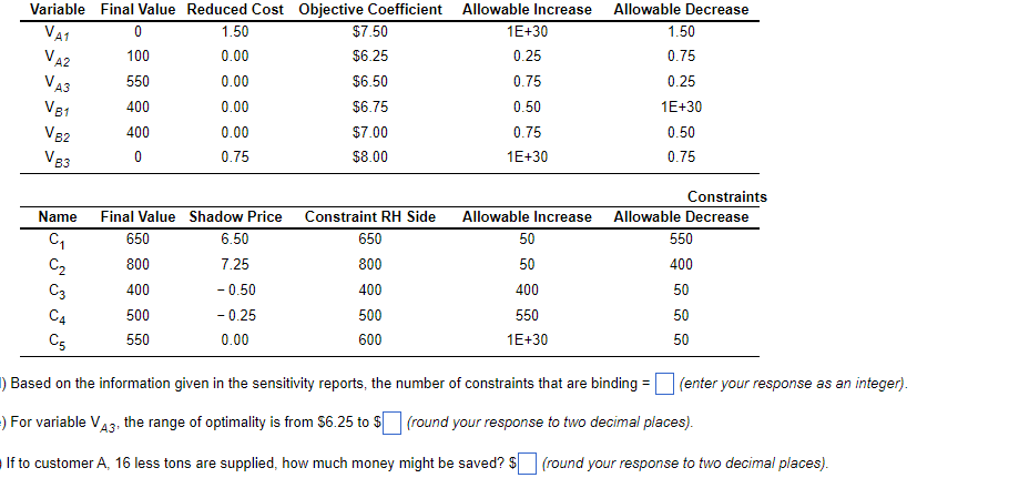
Transcribed Image Text:Allowable Decrease
Variable Final Value Reduced Cost Objective Coefficient
1.50
Allowable Increase
$7.50
1E+30
1.50
VA1
0.00
$6.25
0.25
0.75
100
VA3
$6.50
0.75
0.25
550
0.00
V81
0.00
$6.75
0.50
1E+30
400
0.00
$7.00
0.75
0.50
V82
400
0.75
$8.00
1E+30
0.75
V83
Constraints
Constraint RH Side
Allowable Increase
Allowable Decrease
Name
Final Value Shadow Price
6.50
650
50
550
650
7.25
800
50
400
C2
800
- 0.50
400
50
400
C3
400
C4
- 0.25
500
550
50
500
C5
550
0.00
600
1E+30
50
(enter your response as an integer).
) Based on the information given in the sensitivity reports, the number of constraints that are binding =
) For variable V43. the range of optimality is from $6.25 to $ (round your response to two decimal places).
(round your response to two decimal places).
If to customer A, 16 less tons are supplied, how much money might be saved? $
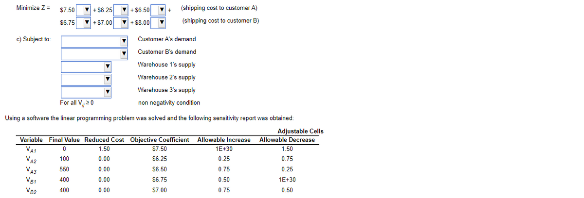
Transcribed Image Text:Minimize Z =
$7.50
V+ $6.25
V + $6.50
(shipping cost to customer A)
$6.75
V + S7.00
V + $8.00
(shipping cost to customer B)
c) Subject to:
Customer A's demand
Customer B's demand
Warehouse 1's supply
Warehouse 2's supply
Warehouse 3's supply
For all Vj 20
non negativity condition
Using a software the linear programming problem was solved and the following sensitivity report was obtained:
Adjustable Cells
Variable Final Value Reduced Cost Objective Coefficient Allowable Increase Allowable Decrease
VA1
1.50
$7.50
1E+30
1.50
V42
100
0.00
$6.25
0.25
0.75
VA3
550
0.00
$6.50
0.75
0.25
V81
V82
400
0.00
$6.75
0.50
1E+30
400
0.00
$7.00
0.75
0.50
Expert Solution
This question has been solved!
Explore an expertly crafted, step-by-step solution for a thorough understanding of key concepts.

This is a popular solution!

Trending now
This is a popular solution!

Step by step
Solved in 4 steps with 3 images

Recommended textbooks for you
Practical Management Science
Operations Management
ISBN:
9781337406659
Author:
WINSTON, Wayne L.
Publisher:
Cengage,
Practical Management Science
Operations Management
ISBN:
9781337406659
Author:
WINSTON, Wayne L.
Publisher:
Cengage,