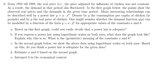
From 1950 till 1988, the real price (i.e., the price adjusted for inflation) of chicken was not constant. As a result, the demand in that period also fluctuated. In the first graph below, the points show the observed real prices and the demands in the given time period. Many interesting relationships can be described well by a power law y = a.2. Denote by q the consumption per capita of chicken (in pounds) and by p the real price of chicken. One might wonder whether the demand function q(p) can be modelled by a function of the form q = a-p for appropriate values of the constants a and b. a. Based on this first graph, could you easily decide that a power law is adequate? b. If you express a power law using logarithmic scales on both axes, what does the graph look like? Explain why this is so. What is the (geometric) meaning of the constants a and b? c. In the second graph below, we show the above data using logarithmic scales on both axes. Based on this, do you think a power law is adequate for the given data?
From 1950 till 1988, the real price (i.e., the price adjusted for inflation) of chicken was not constant. As a result, the demand in that period also fluctuated. In the first graph below, the points show the observed real prices and the demands in the given time period. Many interesting relationships can be described well by a power law y = a.2. Denote by q the consumption per capita of chicken (in pounds) and by p the real price of chicken. One might wonder whether the demand function q(p) can be modelled by a function of the form q = a-p for appropriate values of the constants a and b. a. Based on this first graph, could you easily decide that a power law is adequate? b. If you express a power law using logarithmic scales on both axes, what does the graph look like? Explain why this is so. What is the (geometric) meaning of the constants a and b? c. In the second graph below, we show the above data using logarithmic scales on both axes. Based on this, do you think a power law is adequate for the given data?

Algebra & Trigonometry with Analytic Geometry
13th Edition
ISBN:9781133382119
Author:Swokowski
Publisher:Swokowski
Chapter5: Inverse, Exponential, And Logarithmic Functions
Section5.6: Exponential And Logarithmic Equations
Problem 64E

Related questions
Question
Transcribed Image Text:9. From 1950 till 1988, the real price (i.e., the price adjusted for inflation) of chicken was not constant.
As a result, the demand in that period also fluctuated. In the first graph below, the points show the
observed real prices and the demands in the given time period. Many interesting relationships can
be described well by a power law y = a 2. Denote by q the consumption per capita of chicken (in
pounds) and by p the real price of chicken. One might wonder whether the demand function q(p) can
be modelled by a function of the form q = ap for appropriate values of the constants a and b.
a. Based on this first graph, could you easily decide that a power law is adequate?
b. If you express a power law using logarithmic scales on both axes, what does the graph look like?
Explain why this is so. What is the (geometric) meaning of the constants a and b?
c. In the second graph below, we show the above data using logarithmic scales on both axes. Based
on this, do you think a power law is adequate for the given data?
d. Estimate a and b based on the second graph.
e. Interpret b in the economical context.
Expert Solution
This question has been solved!
Explore an expertly crafted, step-by-step solution for a thorough understanding of key concepts.

Step by step
Solved in 4 steps with 2 images

Recommended textbooks for you
Algebra & Trigonometry with Analytic Geometry
Algebra
ISBN:
9781133382119
Author:
Swokowski
Publisher:
Cengage
Algebra & Trigonometry with Analytic Geometry
Algebra
ISBN:
9781133382119
Author:
Swokowski
Publisher:
Cengage