Hello! I need help explaining the whole procedure, the meaning of the graphs and theorems (images) and how the final result was obtained Thanks
Hello! I need help explaining the whole procedure, the meaning of the graphs and theorems (images) and how the final result was obtained Thanks

A First Course in Probability (10th Edition)
10th Edition
ISBN:9780134753119
Author:Sheldon Ross
Publisher:Sheldon Ross
Chapter1: Combinatorial Analysis
Section: Chapter Questions
Problem 1.1P: a. How many different 7-place license plates are possible if the first 2 places are for letters and...

Related questions
Question
Hello! I need help explaining the whole procedure, the meaning of the graphs and theorems (images) and how the final result was obtained
Thanks
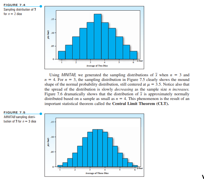
Transcribed Image Text:FIGURE 7.4
Sampling distribution of
for n = 2 dice
FIGURE 7.5
MINITAB sampling distri-
bution of x for n = 3 dice
p(x-bar)
.15-
p(x-bar)
.10-
.05-
0
Using MINITAB, we generated the sampling distributions of when n = 3 and
n = 4. For n = 3, the sampling distribution in Figure 7.5 clearly shows the mound
shape of the normal probability distribution, still centered at μ = 3.5. Notice also that
the spread of the distribution is slowly decreasing as the sample size n increases.
Figure 7.6 dramatically shows that the distribution of is approximately normally
distributed based on a sample as small as n = 4. This phenomenon is the result of an
important statistical theorem called the Central Limit Theorem (CLT).
15-
.10-
.05-
0
Average of Two Dice
2
4
Average of Three Dice
5
x-bar
6
x-bar
Transcribed Image Text:1.4
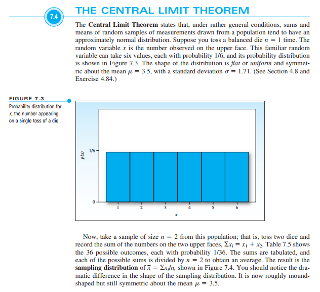
FIGURE 7.3
Probability distribution for
x, the number appearing
on a single toss of a die
THE CENTRAL LIMIT THEOREM
The Central Limit Theorem states that, under rather general conditions, sums and
means of random samples of measurements drawn from a population tend to have an
approximately normal distribution. Suppose you toss a balanced die n = 1 time. The
random variable x is the number observed on the upper face. This familiar random
variable can take six values, each with probability 1/6, and its probability distribution
is shown in Figure 7.3. The shape of the distribution is flat or uniform and symmet-
ric about the mean = 3.5, with a standard deviation = 1.71. (See Section 4.8 and
Exercise 4.84.)
p(x)
1/6-
0
2
x
Now, take a sample of size n = 2 from this population; that is, toss two dice and
record the sum of the numbers on the two upper faces, Ex; = x₁ + x₂. Table 7.5 shows
the 36 possible outcomes, each with probability 1/36. The sums are tabulated, and
each of the possible sums is divided by n = 2 to obtain an average. The result is the
sampling distribution of x = Ex/n, shown in Figure 7.4. You should notice the dra-
matic difference in the shape of the sampling distribution. It is now roughly mound-
shaped but still symmetric about the mean μ = 3.5.
Expert Solution
This question has been solved!
Explore an expertly crafted, step-by-step solution for a thorough understanding of key concepts.

Step by step
Solved in 3 steps

Follow-up Questions
Read through expert solutions to related follow-up questions below.
Follow-up Question
Hi! from the previous explanation I have doubts about how the probabilities of the table are found when using 1,2 and 3 dice. Why is p(x) decreasing as x increases?
Solution
Recommended textbooks for you
A First Course in Probability (10th Edition)
Probability
ISBN:
9780134753119
Author:
Sheldon Ross
Publisher:
PEARSON

A First Course in Probability (10th Edition)
Probability
ISBN:
9780134753119
Author:
Sheldon Ross
Publisher:
PEARSON