In [5]: x_fit = np.linspace(0,21,1000) y_fit = x_fit #Reshape the x fit and y_fit... x_fit = x_fit.reshape(-1,1) y_fit = y_fit.reshape(-1,1) #Fit the model on x fit and y_fit... model.fit(x_fit, y_fit) #Now, merge the x fit and y_fit as dataframe... mixData = pd.DataFrame({'x': [x_fit], 'y': [y_fit]}) #Now, use the predict() method to find the z_fit using the above dataframe... z_fit = model.predict (mixData['x'][0]) Recreate the first image, but plot the line of best fit in each of the subplots as well. In [9]: fig-plt.figure(figsize=[10,10]) #==‒‒‒‒‒‒‒========= # First subplot ======= #set up the axes for the first plot ax1 = fig.add_subplot (2, 2, 1, projection="3d") ax1.scatter(dfData['x'], dfData['y'],dfData['z'],c=dfData['z'],cmap='jet') ax1.set_xlabel('x', fontsize=9) axl.set_ylabel('y', fontsize=9) axl.set_zlabel('z', fontsize=9) axi.view_init(9, 90) start, end = ax1.get_xlim() axi.xaxis.set_ticks(np.arange(0, end, 5)) start2, end2 = axi.get_ylim() axi.yaxis.set_ticks(np.arange(0, end2, 5)) font = {'size': 8} axi.tick_params ('x', labelsize-font['size']) axi.tick_params ('y', labelsize-font['size']) axi.tick_params ('z', labelsize-font['size']) axi.plot3d(x_fit, z_fit, c='black')
In [5]: x_fit = np.linspace(0,21,1000) y_fit = x_fit #Reshape the x fit and y_fit... x_fit = x_fit.reshape(-1,1) y_fit = y_fit.reshape(-1,1) #Fit the model on x fit and y_fit... model.fit(x_fit, y_fit) #Now, merge the x fit and y_fit as dataframe... mixData = pd.DataFrame({'x': [x_fit], 'y': [y_fit]}) #Now, use the predict() method to find the z_fit using the above dataframe... z_fit = model.predict (mixData['x'][0]) Recreate the first image, but plot the line of best fit in each of the subplots as well. In [9]: fig-plt.figure(figsize=[10,10]) #==‒‒‒‒‒‒‒========= # First subplot ======= #set up the axes for the first plot ax1 = fig.add_subplot (2, 2, 1, projection="3d") ax1.scatter(dfData['x'], dfData['y'],dfData['z'],c=dfData['z'],cmap='jet') ax1.set_xlabel('x', fontsize=9) axl.set_ylabel('y', fontsize=9) axl.set_zlabel('z', fontsize=9) axi.view_init(9, 90) start, end = ax1.get_xlim() axi.xaxis.set_ticks(np.arange(0, end, 5)) start2, end2 = axi.get_ylim() axi.yaxis.set_ticks(np.arange(0, end2, 5)) font = {'size': 8} axi.tick_params ('x', labelsize-font['size']) axi.tick_params ('y', labelsize-font['size']) axi.tick_params ('z', labelsize-font['size']) axi.plot3d(x_fit, z_fit, c='black')

Computer Networking: A Top-Down Approach (7th Edition)
7th Edition
ISBN:9780133594140
Author:James Kurose, Keith Ross
Publisher:James Kurose, Keith Ross
Chapter1: Computer Networks And The Internet
Section: Chapter Questions
Problem R1RQ: What is the difference between a host and an end system? List several different types of end...

Related questions
Question
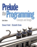
How do I get the line of best fit plotted in my 3D scatterplot in Matlibplot? I am trying to use "plot3d()" but I do not know what to put in the paretheses? To be clear, we HAVE to use x_fit, y_fit and z_fit. Please look at my code and let me know how to get the line plotted in the scatterplot I created - because as you can see, I tried "ax.plot3d(x_fit, z_fit,c='black') but that does not work for me.
![In [5]:
x_fit = np.linspace(0,21,1000)
y_fit = x_fit
#Reshape the x fit and y_fit...
x_fit x_fit.reshape(-1,1)
y_fit = y_fit.reshape(-1,1)
#Fit the model on x_fit and y_fit...
model.fit(x_fit, y_fit)
#Now, merge the x fit and y_fit as dataframe...
mixData = pd.DataFrame({'x': [x_fit], 'y': [y_fit]})
#Now, use the predict() method to find the z_fit using the above dataframe...
z_fit = model.predict(mixData['x'][0])
Recreate the first image, but plot the line of best fit in each of the subplots as well.
In [9]: fig-plt.figure(figsize=[10,10])
#=======
# First subplot
#==========/
====
# set up the axes for the first plot
ax1 = fig.add_subplot(2, 2, 1, projection='3d')
ax1.scatter (dfData['x'], dfData['y'],dfData['z'],c=dfData['z'],cmap='jet')
axl.set_xlabel('x', fontsize=9)
axl.set_ylabel('y', fontsize=9)
axl.set_zlabel('z', fontsize=9)
ax1.view_init(9, 90)
end, 5))
start, end = ax1.get_xlim()
ax1.xaxis.set_ticks(np.arange(0,
start2, end2 = ax1.get_ylim()
ax1.yaxis.set_ticks(np.arange(0, end2, 5))
font = {'size': 8}
ax1.tick_params ('x', labelsize-font['size'])
ax1.tick_params ('y', labelsize-font['size'])
ax1.tick_params ('z', labelsize=font['size'])
ax1.plot3d(x_fit, z_fit, c='black')](/v2/_next/image?url=https%3A%2F%2Fcontent.bartleby.com%2Fqna-images%2Fquestion%2Fe625cb9f-976b-4a6b-8e90-26fc2431c5a0%2Fbc5734f3-a01b-4f8f-a81a-aef1ffc8a096%2F11ef99_processed.png&w=3840&q=75)
Transcribed Image Text:In [5]:
x_fit = np.linspace(0,21,1000)
y_fit = x_fit
#Reshape the x fit and y_fit...
x_fit x_fit.reshape(-1,1)
y_fit = y_fit.reshape(-1,1)
#Fit the model on x_fit and y_fit...
model.fit(x_fit, y_fit)
#Now, merge the x fit and y_fit as dataframe...
mixData = pd.DataFrame({'x': [x_fit], 'y': [y_fit]})
#Now, use the predict() method to find the z_fit using the above dataframe...
z_fit = model.predict(mixData['x'][0])
Recreate the first image, but plot the line of best fit in each of the subplots as well.
In [9]: fig-plt.figure(figsize=[10,10])
#=======
# First subplot
#==========/
====
# set up the axes for the first plot
ax1 = fig.add_subplot(2, 2, 1, projection='3d')
ax1.scatter (dfData['x'], dfData['y'],dfData['z'],c=dfData['z'],cmap='jet')
axl.set_xlabel('x', fontsize=9)
axl.set_ylabel('y', fontsize=9)
axl.set_zlabel('z', fontsize=9)
ax1.view_init(9, 90)
end, 5))
start, end = ax1.get_xlim()
ax1.xaxis.set_ticks(np.arange(0,
start2, end2 = ax1.get_ylim()
ax1.yaxis.set_ticks(np.arange(0, end2, 5))
font = {'size': 8}
ax1.tick_params ('x', labelsize-font['size'])
ax1.tick_params ('y', labelsize-font['size'])
ax1.tick_params ('z', labelsize=font['size'])
ax1.plot3d(x_fit, z_fit, c='black')
Expert Solution
This question has been solved!
Explore an expertly crafted, step-by-step solution for a thorough understanding of key concepts.

This is a popular solution!

Trending now
This is a popular solution!

Step by step
Solved in 2 steps with 2 images

Follow-up Questions
Read through expert solutions to related follow-up questions below.
Follow-up Question
I need the line to be a thin black line so the scatterplot does not "disappear". How to I format it?
Solution
Recommended textbooks for you
Computer Networking: A Top-Down Approach (7th Edi…
Computer Engineering
ISBN:
9780133594140
Author:
James Kurose, Keith Ross
Publisher:
PEARSON

Computer Organization and Design MIPS Edition, Fi…
Computer Engineering
ISBN:
9780124077263
Author:
David A. Patterson, John L. Hennessy
Publisher:
Elsevier Science

Network+ Guide to Networks (MindTap Course List)
Computer Engineering
ISBN:
9781337569330
Author:
Jill West, Tamara Dean, Jean Andrews
Publisher:
Cengage Learning
Computer Networking: A Top-Down Approach (7th Edi…
Computer Engineering
ISBN:
9780133594140
Author:
James Kurose, Keith Ross
Publisher:
PEARSON
Computer Organization and Design MIPS Edition, Fi…
Computer Engineering
ISBN:
9780124077263
Author:
David A. Patterson, John L. Hennessy
Publisher:
Elsevier Science
Network+ Guide to Networks (MindTap Course List)
Computer Engineering
ISBN:
9781337569330
Author:
Jill West, Tamara Dean, Jean Andrews
Publisher:
Cengage Learning

Concepts of Database Management
Computer Engineering
ISBN:
9781337093422
Author:
Joy L. Starks, Philip J. Pratt, Mary Z. Last
Publisher:
Cengage Learning
Prelude to Programming
Computer Engineering
ISBN:
9780133750423
Author:
VENIT, Stewart
Publisher:
Pearson Education

Sc Business Data Communications and Networking, T…
Computer Engineering
ISBN:
9781119368830
Author:
FITZGERALD
Publisher:
WILEY