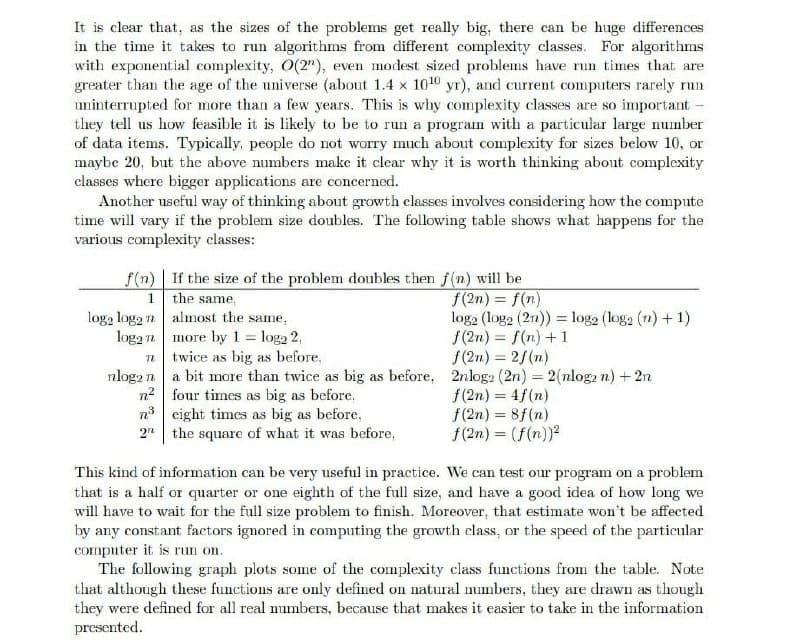
It is clear that, as the sizes of the problems get really big, there can be huge differences in the time it takes to run algorithms from different complexity classes. For algorithms with exponential complexity, O(2"), even modest sized problems have run times that are greater than the age of the universe (about 1.4 x 10¹⁰ yr), and current computers rarely run uninterrupted for more than a few years. This is why complexity classes are so important - they tell us how feasible it is likely to be to run a program with a particular large number of data items. Typically, people do not worry much about complexity for sizes below 10, or maybe 20, but the above numbers make it clear why it is worth thinking about complexity classes where bigger applications are concerned. Another useful way of thinking about growth classes involves considering how the compute time will vary if the problem size doubles. The following table shows what happens for the various complexity classes: f(n) | If the size of the problem doubles then f(n) will be 1 the same, loga log2 n almost the same, log2 n more by = log2 2, n twice as big as before, nlog2 n a bit more than twice as big as before, 2nlog2 (2n) = 2(nlog2 n) + 2n n2 four times as big as before, n eight times as big as before, 2" the square of what it was before, f(2n) = f(n) loga (log2 (2n)) = log2 (log2 (n) + 1) f(2n) = f(n) +1 f(2n) = 2f(n) %3D f(2n) = 4f(n) f(2n) = 8f(n) f(2n) = (f(n))? This kind of information can be very useful in practice. We can test our program on a problem that is a half or quarter or one eighth of the full size, and have a good idea of how long we will have to wait for the full size problem to finish. Moreover, that estimate won't be affected by any constant factors ignored in computing the growth class, or the speed of the particular computer it is run on. The following graph plots some of the complexity class functions from the table. Note that although these functions are only defined on natural mumbers, they are drawn as though they were defined for all real mumbers, because that makes it easier to take in the information presented.
It is clear that, as the sizes of the problems get really big, there can be huge differences in the time it takes to run algorithms from different complexity classes. For algorithms with exponential complexity, O(2"), even modest sized problems have run times that are greater than the age of the universe (about 1.4 x 10¹⁰ yr), and current computers rarely run uninterrupted for more than a few years. This is why complexity classes are so important - they tell us how feasible it is likely to be to run a program with a particular large number of data items. Typically, people do not worry much about complexity for sizes below 10, or maybe 20, but the above numbers make it clear why it is worth thinking about complexity classes where bigger applications are concerned. Another useful way of thinking about growth classes involves considering how the compute time will vary if the problem size doubles. The following table shows what happens for the various complexity classes: f(n) | If the size of the problem doubles then f(n) will be 1 the same, loga log2 n almost the same, log2 n more by = log2 2, n twice as big as before, nlog2 n a bit more than twice as big as before, 2nlog2 (2n) = 2(nlog2 n) + 2n n2 four times as big as before, n eight times as big as before, 2" the square of what it was before, f(2n) = f(n) loga (log2 (2n)) = log2 (log2 (n) + 1) f(2n) = f(n) +1 f(2n) = 2f(n) %3D f(2n) = 4f(n) f(2n) = 8f(n) f(2n) = (f(n))? This kind of information can be very useful in practice. We can test our program on a problem that is a half or quarter or one eighth of the full size, and have a good idea of how long we will have to wait for the full size problem to finish. Moreover, that estimate won't be affected by any constant factors ignored in computing the growth class, or the speed of the particular computer it is run on. The following graph plots some of the complexity class functions from the table. Note that although these functions are only defined on natural mumbers, they are drawn as though they were defined for all real mumbers, because that makes it easier to take in the information presented.

Computer Networking: A Top-Down Approach (7th Edition)
7th Edition
ISBN:9780133594140
Author:James Kurose, Keith Ross
Publisher:James Kurose, Keith Ross
Chapter1: Computer Networks And The Internet
Section: Chapter Questions
Problem R1RQ: What is the difference between a host and an end system? List several different types of end...

Related questions
Question
Plot it
Transcribed Image Text:It is clear that, as the sizes of the problems get really big, there can be huge differences
in the time it takes to run algorithms from different complexity classes. For algorithms
with exponential complexity, O(2"), even modest sized problems have run times that are
greater than the age of the universe (about 1.4 x 10¹⁰ yr), and current computers rarely run
uninterrupted for more than a few years. This is why complexity classes are so important -
they tell us how feasible it is likely to be to run a program with a particular large number
of data items. Typically, people do not worry much about complexity for sizes below 10, or
maybe 20, but the above numbers make it clear why it is worth thinking about complexity
classes where bigger applications are concerned.
Another useful way of thinking about growth classes involves considering how the compute
time will vary if the problem size doubles. The following table shows what happens for the
various complexity classes:
f(n) If the size of the problem doubles then f(n) will be
f(2n) = f(n)
1 the same,
logo loga n almost the same,
loga n more by 1 = log2 2,
twice as big as before,
log2 (log2 (2n)) = logo (log2 (n) + 1)
%3D
f(2n) = f(n) +1
f(2n) = 2f(n)
%3D
nlogz n a bit more than twice as big as before, 2nlog2 (2n) = 2(nlog2 n) + 2n
n2 four times as big as before,
n3 eight times as big as before,
the square of what it was before,
f(2n) = 4f(n)
f(2n) = 8f(n)
f(2n) = (f(n))?
This kind of information can be very useful in practice. We can test our program on a problem
that is a half or quarter or one eighth of the full size, and have a good idea of how long we
will have to wait for the full size problem to finish. Moreover, that estimate won't be affected
by any constant factors ignored in computing the growth class, or the speed of the particular
computer it is run on.
The following graph plots some of the complexity class functions from the table. Note
that although these functions are only defined on natural mumbers, they are drawn as though
they were defined for all real mumbers, because that makes it easier to take in the information
presented.
Expert Solution
This question has been solved!
Explore an expertly crafted, step-by-step solution for a thorough understanding of key concepts.

Step by step
Solved in 2 steps with 1 images

Recommended textbooks for you
Computer Networking: A Top-Down Approach (7th Edi…
Computer Engineering
ISBN:
9780133594140
Author:
James Kurose, Keith Ross
Publisher:
PEARSON

Computer Organization and Design MIPS Edition, Fi…
Computer Engineering
ISBN:
9780124077263
Author:
David A. Patterson, John L. Hennessy
Publisher:
Elsevier Science

Network+ Guide to Networks (MindTap Course List)
Computer Engineering
ISBN:
9781337569330
Author:
Jill West, Tamara Dean, Jean Andrews
Publisher:
Cengage Learning
Computer Networking: A Top-Down Approach (7th Edi…
Computer Engineering
ISBN:
9780133594140
Author:
James Kurose, Keith Ross
Publisher:
PEARSON
Computer Organization and Design MIPS Edition, Fi…
Computer Engineering
ISBN:
9780124077263
Author:
David A. Patterson, John L. Hennessy
Publisher:
Elsevier Science
Network+ Guide to Networks (MindTap Course List)
Computer Engineering
ISBN:
9781337569330
Author:
Jill West, Tamara Dean, Jean Andrews
Publisher:
Cengage Learning
Concepts of Database Management
Computer Engineering
ISBN:
9781337093422
Author:
Joy L. Starks, Philip J. Pratt, Mary Z. Last
Publisher:
Cengage Learning

Prelude to Programming
Computer Engineering
ISBN:
9780133750423
Author:
VENIT, Stewart
Publisher:
Pearson Education

Sc Business Data Communications and Networking, T…
Computer Engineering
ISBN:
9781119368830
Author:
FITZGERALD
Publisher:
WILEY