
Algebra and Trigonometry (MindTap Course List)
4th Edition
ISBN:9781305071742
Author:James Stewart, Lothar Redlin, Saleem Watson
Publisher:James Stewart, Lothar Redlin, Saleem Watson
Chapter2: Functions
Section2.6: Transformations Of Functions
Problem 99E: Field Trip A class of fourth graders walks to a park on a field trip. The function y=f(t) graphed...

Related questions
Question
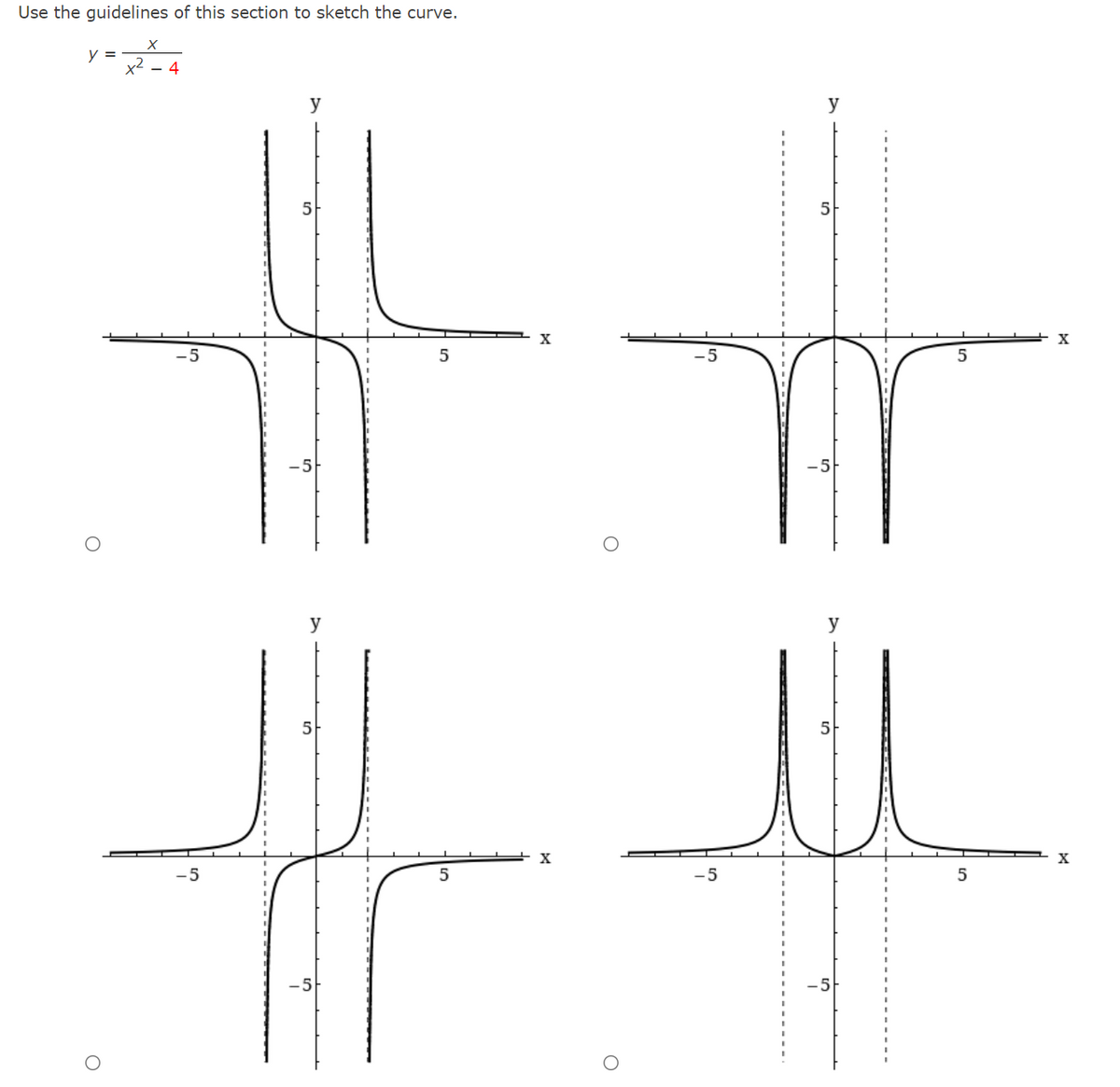
Transcribed Image Text:Use the guidelines of this section to sketch the curve.
y =
x2 - 4
y
y
X
X
-5
5
-5
5
-5
-5
y
5
5
-5
-5
-5
-5
![Guidelines for Sketching a Curve
The following checklist is intended as a guide to sketching a curve y = f(x) by hand. Not
every item is relevant to every function. (For instance, a given curve might not have an
asymptote or possess symmetry.) But the guidelines provide all the information you need
to make a sketch that displays the most important aspects of the function.
A. Domain It's often useful to start by determining the domain D of f, that is, the set of
values of x for which f(x) is defined.
B. Intercepts The y-intercept is f(0) and this tells us where the curve intersects the y-axis.
To find the x-intercepts,
tion is difficult to solve.)
C. Symmetry
set y = 0 and solve for x. (You can omit this step if the equa-
(i) If f(-x) = f(x) for all x in D, that is, the equation of the curve is unchanged
when x is replaced by -x, then f is an even function and the curve is symmetric about
the y-axis. This means that our work is cut in half. If we know what the curve looks like
for x> 0, then we need only reflect about the y-axis to obtain the complete curve [see
Figure 1(a)]. Here are some examples: y = x², y = x*, y = |x|, and y = cos x.
(a) Even function: reflectional symmetry
(ii) If f(-x) = -f(x) for all x in D, then f is an odd function and the curve is sym-
metric about the origin. Again we can obtain the complete curve if we know what it looks
like for x > 0. [Rotate 180° about the origin; see Figure 1(b).] Some simple examples
of odd functions are y = x, y = x°, y = x', and y = sin x.
( iii) If f(x + p) = f(x) for all x in D, where p is a positive constant, then f is called
a periodic function and the smallest such number p is called the period. For instance,
y = sin x has period 27 and y = tan x has period T. If we know what the graph looks
like in an interval of length p, then we can use translation to sketch the entire graph (see
Figure 2).
(b) Odd function: rotational symmetry
FIGURE 1
FIGURE 2
Periodic function:
translational symmetry
а -р
a +p
a + 2p
a
D. Asymptotes
(i) Horizontal Asymptotes. Recall from Section 2.6 that if either lim, f(x) = L
or limx--« f(x) = L, then the line y = L is a horizontal asymptote of the curve y = f(x).
If it turns out that lim, f(x) = 0 (or -0), then we do not have an asymptote to the
right, but that is still useful information for sketching the curve.
(ii) Vertical Asymptotes. Recall from Section 2.2 that the line x = a is a vertical
asymptote if at least one of the following statements is true:
1
lim f(x) = o
lim f(x) = 0
Xa+
Xa-
lim f(x) = -00
lim f(x) = -0
(For rational functions you can locate the vertical asymptotes by equating the denomi-
nator to 0 after canceling any common factors. But for other functions this method does
not apply.) Furthermore, in sketching the curve it is very useful to know exactly which
of the statements in [1 is true. If f(a) is not defined but a is an endpoint of the domain
of f, then you should compute lim,a-f(x) or lim,a+ f(x), whether or not this limit is
infinite.
(iii) Slant Asymptotes. These are discussed at the end of this section.
E. Intervals of Increase or Decrease Use the I/D Test. Compute f'(x) and find the intervals
on which f(x) is positive (f is increasing) and the intervals on which f'(x) is negative
(f is decreasing).
F. Local Maximum and Minimum Values Find the critical numbers of f [the numbers c where
f'(c) = 0 or f'(c) does not exist]. Then use the First Derivative Test. If f' changes from
positive to negative at a critical number c, then f (c) is a local maximum. If f' changes
from negative to positive at c, then f(c) is a local minimum. Although it is usually prefer-
able to use the First Derivative Test, you can use the Second Derivative Test if f'(c) = 0
and f"(c) + 0. Then f "(c) > 0 implies that f(c) is a local minimum, whereas f"(c) <0
implies that f(c) is a local maximum.
G. Concavity and Points of Inflection Compute f"(x) and use the Concavity Test. The curve
is concave upward where f"(x) > 0 and concave downward where f"(x) < 0. Inflec-
tion points occur where the direction of concavity changes.
H. Sketch the Curve Using the information in items A-G, draw the graph. Sketch the
asymptotes as dashed lines. Plot the intercepts, maximum and minimum points, and
inflection points. Then make the curve pass through these points, rising and falling
according to E, with concavity according to G, and approaching the asymptotes. If
additional accuracy is desired near any point, you can compute the value of the derivative
there. The tangent indicates the direction in which the curve proceeds.](/v2/_next/image?url=https%3A%2F%2Fcontent.bartleby.com%2Fqna-images%2Fquestion%2F5a91dce2-7b78-488c-a950-bff9db4e775f%2F87dc36a5-8558-4c4f-bea2-646fc9b709e7%2Fi25xyas_processed.gif&w=3840&q=75)
Transcribed Image Text:Guidelines for Sketching a Curve
The following checklist is intended as a guide to sketching a curve y = f(x) by hand. Not
every item is relevant to every function. (For instance, a given curve might not have an
asymptote or possess symmetry.) But the guidelines provide all the information you need
to make a sketch that displays the most important aspects of the function.
A. Domain It's often useful to start by determining the domain D of f, that is, the set of
values of x for which f(x) is defined.
B. Intercepts The y-intercept is f(0) and this tells us where the curve intersects the y-axis.
To find the x-intercepts,
tion is difficult to solve.)
C. Symmetry
set y = 0 and solve for x. (You can omit this step if the equa-
(i) If f(-x) = f(x) for all x in D, that is, the equation of the curve is unchanged
when x is replaced by -x, then f is an even function and the curve is symmetric about
the y-axis. This means that our work is cut in half. If we know what the curve looks like
for x> 0, then we need only reflect about the y-axis to obtain the complete curve [see
Figure 1(a)]. Here are some examples: y = x², y = x*, y = |x|, and y = cos x.
(a) Even function: reflectional symmetry
(ii) If f(-x) = -f(x) for all x in D, then f is an odd function and the curve is sym-
metric about the origin. Again we can obtain the complete curve if we know what it looks
like for x > 0. [Rotate 180° about the origin; see Figure 1(b).] Some simple examples
of odd functions are y = x, y = x°, y = x', and y = sin x.
( iii) If f(x + p) = f(x) for all x in D, where p is a positive constant, then f is called
a periodic function and the smallest such number p is called the period. For instance,
y = sin x has period 27 and y = tan x has period T. If we know what the graph looks
like in an interval of length p, then we can use translation to sketch the entire graph (see
Figure 2).
(b) Odd function: rotational symmetry
FIGURE 1
FIGURE 2
Periodic function:
translational symmetry
а -р
a +p
a + 2p
a
D. Asymptotes
(i) Horizontal Asymptotes. Recall from Section 2.6 that if either lim, f(x) = L
or limx--« f(x) = L, then the line y = L is a horizontal asymptote of the curve y = f(x).
If it turns out that lim, f(x) = 0 (or -0), then we do not have an asymptote to the
right, but that is still useful information for sketching the curve.
(ii) Vertical Asymptotes. Recall from Section 2.2 that the line x = a is a vertical
asymptote if at least one of the following statements is true:
1
lim f(x) = o
lim f(x) = 0
Xa+
Xa-
lim f(x) = -00
lim f(x) = -0
(For rational functions you can locate the vertical asymptotes by equating the denomi-
nator to 0 after canceling any common factors. But for other functions this method does
not apply.) Furthermore, in sketching the curve it is very useful to know exactly which
of the statements in [1 is true. If f(a) is not defined but a is an endpoint of the domain
of f, then you should compute lim,a-f(x) or lim,a+ f(x), whether or not this limit is
infinite.
(iii) Slant Asymptotes. These are discussed at the end of this section.
E. Intervals of Increase or Decrease Use the I/D Test. Compute f'(x) and find the intervals
on which f(x) is positive (f is increasing) and the intervals on which f'(x) is negative
(f is decreasing).
F. Local Maximum and Minimum Values Find the critical numbers of f [the numbers c where
f'(c) = 0 or f'(c) does not exist]. Then use the First Derivative Test. If f' changes from
positive to negative at a critical number c, then f (c) is a local maximum. If f' changes
from negative to positive at c, then f(c) is a local minimum. Although it is usually prefer-
able to use the First Derivative Test, you can use the Second Derivative Test if f'(c) = 0
and f"(c) + 0. Then f "(c) > 0 implies that f(c) is a local minimum, whereas f"(c) <0
implies that f(c) is a local maximum.
G. Concavity and Points of Inflection Compute f"(x) and use the Concavity Test. The curve
is concave upward where f"(x) > 0 and concave downward where f"(x) < 0. Inflec-
tion points occur where the direction of concavity changes.
H. Sketch the Curve Using the information in items A-G, draw the graph. Sketch the
asymptotes as dashed lines. Plot the intercepts, maximum and minimum points, and
inflection points. Then make the curve pass through these points, rising and falling
according to E, with concavity according to G, and approaching the asymptotes. If
additional accuracy is desired near any point, you can compute the value of the derivative
there. The tangent indicates the direction in which the curve proceeds.
Expert Solution
This question has been solved!
Explore an expertly crafted, step-by-step solution for a thorough understanding of key concepts.

This is a popular solution!

Trending now
This is a popular solution!

Step by step
Solved in 2 steps

Recommended textbooks for you
Algebra and Trigonometry (MindTap Course List)
Algebra
ISBN:
9781305071742
Author:
James Stewart, Lothar Redlin, Saleem Watson
Publisher:
Cengage Learning

Algebra & Trigonometry with Analytic Geometry
Algebra
ISBN:
9781133382119
Author:
Swokowski
Publisher:
Cengage

College Algebra
Algebra
ISBN:
9781305115545
Author:
James Stewart, Lothar Redlin, Saleem Watson
Publisher:
Cengage Learning
Algebra and Trigonometry (MindTap Course List)
Algebra
ISBN:
9781305071742
Author:
James Stewart, Lothar Redlin, Saleem Watson
Publisher:
Cengage Learning
Algebra & Trigonometry with Analytic Geometry
Algebra
ISBN:
9781133382119
Author:
Swokowski
Publisher:
Cengage
College Algebra
Algebra
ISBN:
9781305115545
Author:
James Stewart, Lothar Redlin, Saleem Watson
Publisher:
Cengage Learning

Elementary Linear Algebra (MindTap Course List)
Algebra
ISBN:
9781305658004
Author:
Ron Larson
Publisher:
Cengage Learning