location to meet. Your positions at time t are denoted by x1(t) and x2(t), and are real valued. Both of you do not have a GPS device and can only measure the relative distance between each other. (a) equation Construct two functions (or strategies) R1(y) and R2(y) such that for the differential dx1 R1 (x1 – x2) (3) dt dx2 R2 (®1 – 22) (4) %3D dt we get lim0 |x1(t) – x2(t)| = 0, irrespective of your initial positions x1(0) and x2(0). Note: R1(y) and R2(y) should not depend on your initial positions (because you don't have GPS). Additionally, note that the right hand-side in Equation (3) means we are evaluating R1(y) at y = xı – x2 and similarly, we are evaulating R2(y) at y = x1 – x2. (b) tancing and maintain p units distance at equilibrium. Modify your functions R1(y) and R2(y) so that lim0 |æ1(t) – x2(t)| = p, irrespective of your initial positions x1(0) and x2(0). As in Consider the alternative scenario that you and your friend must practice social dis- part o) R. (4) and Rolu) should not denend on vour initial positions
location to meet. Your positions at time t are denoted by x1(t) and x2(t), and are real valued. Both of you do not have a GPS device and can only measure the relative distance between each other. (a) equation Construct two functions (or strategies) R1(y) and R2(y) such that for the differential dx1 R1 (x1 – x2) (3) dt dx2 R2 (®1 – 22) (4) %3D dt we get lim0 |x1(t) – x2(t)| = 0, irrespective of your initial positions x1(0) and x2(0). Note: R1(y) and R2(y) should not depend on your initial positions (because you don't have GPS). Additionally, note that the right hand-side in Equation (3) means we are evaluating R1(y) at y = xı – x2 and similarly, we are evaulating R2(y) at y = x1 – x2. (b) tancing and maintain p units distance at equilibrium. Modify your functions R1(y) and R2(y) so that lim0 |æ1(t) – x2(t)| = p, irrespective of your initial positions x1(0) and x2(0). As in Consider the alternative scenario that you and your friend must practice social dis- part o) R. (4) and Rolu) should not denend on vour initial positions

Algebra & Trigonometry with Analytic Geometry
13th Edition
ISBN:9781133382119
Author:Swokowski
Publisher:Swokowski
Chapter5: Inverse, Exponential, And Logarithmic Functions
Section5.6: Exponential And Logarithmic Equations
Problem 64E

Related questions

Concept explainers
Contingency Table
A contingency table can be defined as the visual representation of the relationship between two or more categorical variables that can be evaluated and registered. It is a categorical version of the scatterplot, which is used to investigate the linear relationship between two variables. A contingency table is indeed a type of frequency distribution table that displays two variables at the same time.
Binomial Distribution
Binomial is an algebraic expression of the sum or the difference of two terms. Before knowing about binomial distribution, we must know about the binomial theorem.
Topic Video
Question
PART A
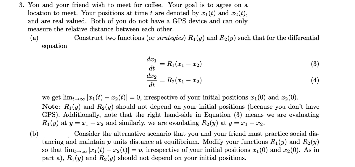
Transcribed Image Text:3. You and your friend wish to meet for coffee. Your goal is to agree on a
location to meet. Your positions at time t are denoted by x1(t) and x2(t),
and are real valued. Both of you do not have a GPS device and can only
measure the relative distance between each other.
(a)
equation
Construct two functions (or strategies) R1 (y) and R2(y) such that for the differential
dx1
= R1 (x1 – x2)
(3)
dt
dx2
R2 (x1 – x2)
(4)
dt
we get lim,→0 |¤1(t) – x2(t)| = 0, irrespective of your initial positions x1(0) and x2(0).
Note: R1(y) and R2(y) should not depend on your initial positions (because you don't have
GPS). Additionally, note that the right hand-side in Equation (3) means we are evaluating
R1 (y) at y = x1 – x2 and similarly, we are evaulating R2(y) at y = x1 – x2.
(b)
tancing and maintain p units distance at equilibrium. Modify your functions R1(y) and R2 (y)
so that lim;→0 |x1(t) – x2(t)| = p, irrespective of your initial positions x1 (0) and x2(0). As in
part a), R1(y) and R2(y) should not depend on your initial positions.
Consider the alternative scenario that you and your friend must practice social dis-
Expert Solution
This question has been solved!
Explore an expertly crafted, step-by-step solution for a thorough understanding of key concepts.

Step by step
Solved in 3 steps

Knowledge Booster


Learn more about
Need a deep-dive on the concept behind this application? Look no further. Learn more about this topic, advanced-math and related others by exploring similar questions and additional content below.Recommended textbooks for you
Algebra & Trigonometry with Analytic Geometry
Algebra
ISBN:
9781133382119
Author:
Swokowski
Publisher:
Cengage
Algebra & Trigonometry with Analytic Geometry
Algebra
ISBN:
9781133382119
Author:
Swokowski
Publisher:
Cengage