Often a radical change in the form of the solution of a differential equation corresponds to a very small change in either the initial condition or the equation itself. Find an explicit solution of the given initial-value problem. dy = (y - 1)2 + 0.04, y(0) = 1 dx y = Use a graphing utility to plot the graph of the solution in a neighborhood of (0, 1). Compare the graph with those obtained in Problems 39, 40, and 42 of Section 2.2. y y y 1.0015 1.0015 1.015 1.0010 1.0010 1.010 1.0005 1.0005 1.005 -0.015-0.010-0.005 0.005 0.0100.015 -0.015 -0.010-0.005 0.9995 0.005 0.010 0.015 -0.015-0.010-0.005 0.9995 0.005 0.010 0.015 0.995 0.9990 0.9990 0.990 0.9985 0.9985 0.985 y 1.015 1.010 1.005 -0.015 -0.010-0.005 0.995 0.005 0.010 0.015 0.990 0.985
Often a radical change in the form of the solution of a differential equation corresponds to a very small change in either the initial condition or the equation itself. Find an explicit solution of the given initial-value problem. dy = (y - 1)2 + 0.04, y(0) = 1 dx y = Use a graphing utility to plot the graph of the solution in a neighborhood of (0, 1). Compare the graph with those obtained in Problems 39, 40, and 42 of Section 2.2. y y y 1.0015 1.0015 1.015 1.0010 1.0010 1.010 1.0005 1.0005 1.005 -0.015-0.010-0.005 0.005 0.0100.015 -0.015 -0.010-0.005 0.9995 0.005 0.010 0.015 -0.015-0.010-0.005 0.9995 0.005 0.010 0.015 0.995 0.9990 0.9990 0.990 0.9985 0.9985 0.985 y 1.015 1.010 1.005 -0.015 -0.010-0.005 0.995 0.005 0.010 0.015 0.990 0.985

Calculus: Early Transcendentals
8th Edition
ISBN:9781285741550
Author:James Stewart
Publisher:James Stewart
Chapter1: Functions And Models
Section: Chapter Questions
Problem 1RCC: (a) What is a function? What are its domain and range? (b) What is the graph of a function? (c) How...

Related questions
Question
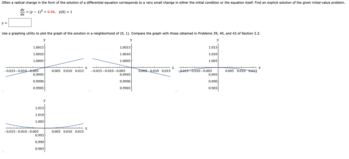
Transcribed Image Text:Often a radical change in the form of the solution of a differential equation corresponds to a very small change in either the initial condition or the equation itself. Find an explicit solution of the given initial-value problem.
dy
= (y – 1)2 + 0.04, y(0) = 1
dx
y =
Use a graphing utility to plot the graph of the solution in a neighborhood of (0, 1). Compare the graph with those obtained in Problems 39, 40, and 42 of Section 2.2.
y
y
y
1.0015
1.0015
1.015
1.0010
1.0010
1.010
1.0005
1.0005
1.005
X
X
-0.015 -0.010-0.005
0.9995
-0.015-0.010–0.005
0.995
0.005 0.010 0.015
-0.015 -0.010-0.005
0.005 0.010 0.015
0.005 0.010 0.015
0.9995
0.9990
0.9990
0.990
0.9985
0.9985
0.985
y
1.015
1.010
1.005
-0.015 –0.010–0.005
0.005 0.010 0.015
0.9
0.990
0.985
Expert Solution
Step 1
First of integrate the given equation as follows

Trending now
This is a popular solution!

Step by step
Solved in 3 steps with 2 images

Recommended textbooks for you
Calculus: Early Transcendentals
Calculus
ISBN:
9781285741550
Author:
James Stewart
Publisher:
Cengage Learning

Thomas' Calculus (14th Edition)
Calculus
ISBN:
9780134438986
Author:
Joel R. Hass, Christopher E. Heil, Maurice D. Weir
Publisher:
PEARSON

Calculus: Early Transcendentals (3rd Edition)
Calculus
ISBN:
9780134763644
Author:
William L. Briggs, Lyle Cochran, Bernard Gillett, Eric Schulz
Publisher:
PEARSON
Calculus: Early Transcendentals
Calculus
ISBN:
9781285741550
Author:
James Stewart
Publisher:
Cengage Learning
Thomas' Calculus (14th Edition)
Calculus
ISBN:
9780134438986
Author:
Joel R. Hass, Christopher E. Heil, Maurice D. Weir
Publisher:
PEARSON
Calculus: Early Transcendentals (3rd Edition)
Calculus
ISBN:
9780134763644
Author:
William L. Briggs, Lyle Cochran, Bernard Gillett, Eric Schulz
Publisher:
PEARSON

Calculus: Early Transcendentals
Calculus
ISBN:
9781319050740
Author:
Jon Rogawski, Colin Adams, Robert Franzosa
Publisher:
W. H. Freeman


Calculus: Early Transcendental Functions
Calculus
ISBN:
9781337552516
Author:
Ron Larson, Bruce H. Edwards
Publisher:
Cengage Learning