Step 3: Find the indicated values and report them below. Regression sum of squares (SSRegr), rounded to four decimal places is 0.8147. degrees of freedom for SSRegr. k= Residual sum of squares (SSResid), rounded to four decimal places is 0.1686. degrees of freedom for SSResid: n - (k+ 1) = [ Compute the F test statistic using the rounded values reported above. (Round the statistic to two decimal places. Note that your number below will not match the F statistic from the output exactly due to using the rounded values above.) SSRegr numerator SSResid df denominator This test statistic has an F probability distribution with df F=- and df denominator" Step 4: The test statistic found in step 3 has a P-value < 0.01 ✓x.(Pick the smallest number the P-value is less than). Thus, there appears to be a useful linear relationship between y and at least one of the three predictors. Provide the linear multiple regression model with all values. (Round the intercept as well as the GPA and Pell Gran coefficients to three decimal places. Round the SAT coefficient to four decimal places.) numerator
Step 3: Find the indicated values and report them below. Regression sum of squares (SSRegr), rounded to four decimal places is 0.8147. degrees of freedom for SSRegr. k= Residual sum of squares (SSResid), rounded to four decimal places is 0.1686. degrees of freedom for SSResid: n - (k+ 1) = [ Compute the F test statistic using the rounded values reported above. (Round the statistic to two decimal places. Note that your number below will not match the F statistic from the output exactly due to using the rounded values above.) SSRegr numerator SSResid df denominator This test statistic has an F probability distribution with df F=- and df denominator" Step 4: The test statistic found in step 3 has a P-value < 0.01 ✓x.(Pick the smallest number the P-value is less than). Thus, there appears to be a useful linear relationship between y and at least one of the three predictors. Provide the linear multiple regression model with all values. (Round the intercept as well as the GPA and Pell Gran coefficients to three decimal places. Round the SAT coefficient to four decimal places.) numerator

A First Course in Probability (10th Edition)
10th Edition
ISBN:9780134753119
Author:Sheldon Ross
Publisher:Sheldon Ross
Chapter1: Combinatorial Analysis
Section: Chapter Questions
Problem 1.1P: a. How many different 7-place license plates are possible if the first 2 places are for letters and...

Related questions
Question
Thank you for any help.
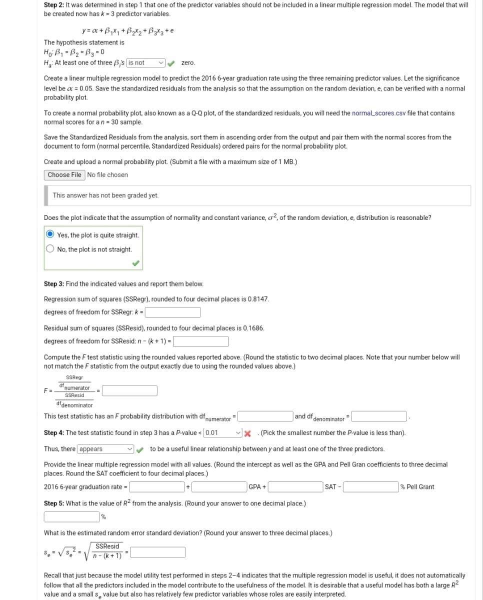
Transcribed Image Text:Step 2: It was determined in step 1 that one of the predictor variables should not be included in a linear multiple regression model. The model that will
be created now has k = 3 predictor variables.
y=x+B₁x₁ +B₂x₂ + B 3x3 + e
The hypothesis statement is
Ho: B₁=B₂=B3 = 0
H: At least one of three B's is not
Create a linear multiple regression model to predict the 2016 6-year graduation rate using the three remaining predictor values. Let the significance
level be x = 0.05. Save the standardized residuals from the analysis so that the assumption on the random deviation, e, can be verified with a normal
probability plot.
zero.
To create a normal probability plot, also known as a Q-Q plot, of the standardized residuals, you will need the normal_scores.csv file that contains
normal scores for a n = 30 sample.
Save the Standardized Residuals from the analysis, sort them in ascending order from the output and pair them with the normal scores from the
document to form (normal percentile, Standardized Residuals) ordered pairs for the normal probability plot.
Create and upload a normal probability plot. (Submit a file with a maximum size of 1 MB.)
Choose File No file chosen
This answer has not been graded yet.
Does the plot indicate that the assumption of normality and constant variance, o2, of the random deviation, e, distribution is reasonable?
Yes, the plot is quite straight.
No, the plot is not straight.
Step 3: Find the indicated values and report them below.
Regression sum of squares (SSRegr), rounded to four decimal places is 0.8147.
degrees of freedom for SSRegr: k =
k=
Residual sum of squares (SSResid), rounded to four decimal places is 0.1686.
degrees of freedom for SSResid: n - (k+ 1) =
Compute the F test statistic using the rounded values reported above. (Round the statistic to two decimal places. Note that your number below will
not match the F statistic from the output exactly due to using the rounded values above.)
SSRegr
F=numerator
SSResid
df denominator
This test statistic has an F probability distribution with df numerator
and df denominator
✓x.(Pick the smallest number the P-value is less than).
Step 4: The test statistic found in step 3 has a P-value < 0.01
Thus, there appears
✓✓to be a useful linear relationship between y and at least one of the three predictors.
Provide the linear multiple regression model with all values. (Round the intercept as well as the GPA and Pell Gran coefficients to three decimal
places. Round the SAT coefficient to four decimal places.)
2016 6-year graduation rate=
Se= √ Se
=
GPA +
Step 5: What is the value of R2 from the analysis. (Round your answer to one decimal place.)
%
SAT
What is the estimated random error standard deviation? (Round your answer to three decimal places.)
SSResid
n-(k+1)=
% Pell Grant
Recall that just because the model utility test performed in steps 2-4 indicates that the multiple regression model is useful, it does not automatically
follow that all the predictors included in the model contribute to the usefulness of the model. It is desirable that a useful model has both a large R²
value and a small s value but also has relatively few predictor variables whose roles are easily interpreted.
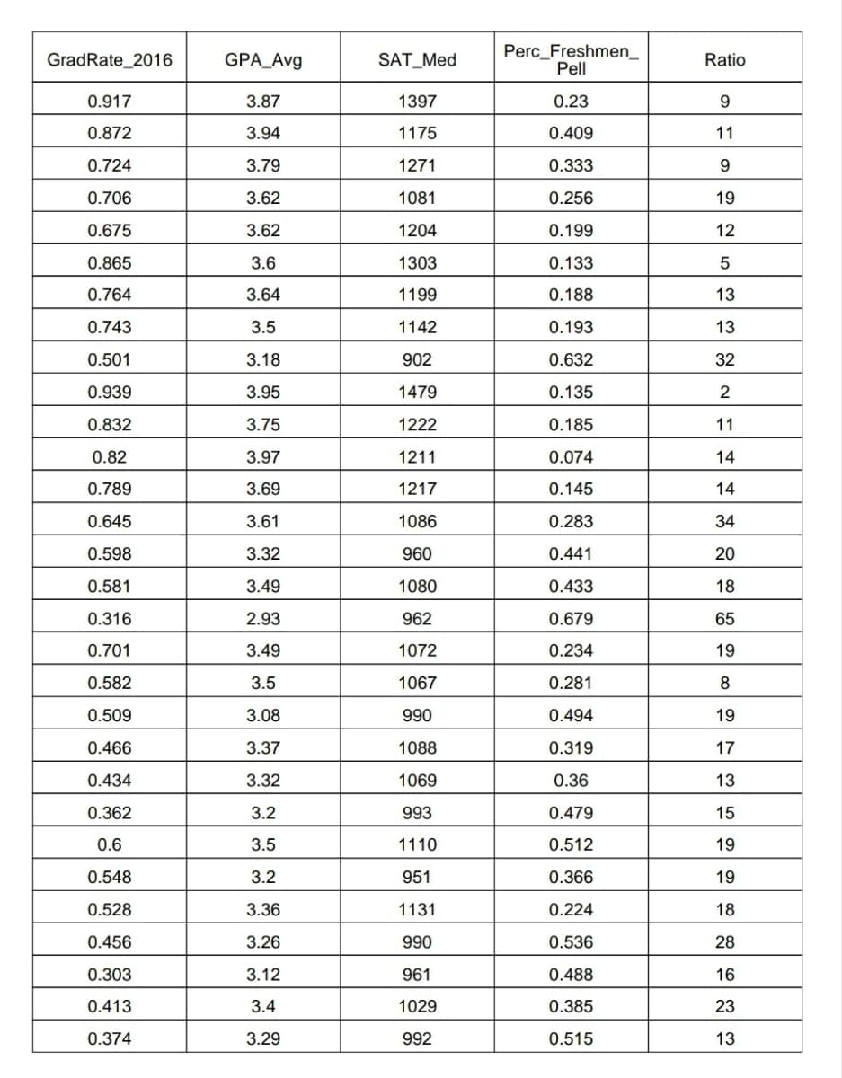
Transcribed Image Text:GradRate_2016
0.917
0.872
0.724
0.706
0.675
0.865
0.764
0.743
0.501
0.939
0.832
0.82
0.789
0.645
0.598
0.581
0.316
0.701
0.582
0.509
0.466
0.434
0.362
0.6
0.548
0.528
0.456
0.303
0.413
0.374
GPA_Avg
3.87
3.94
3.79
3.62
3.62
3.6
3.64
3.5
3.18
3.95
3.75
3.97
3.69
3.61
3.32
3.49
2.93
3.49
3.5
3.08
3.37
3.32
3.2
3.5
3.2
3.36
3.26
3.12
3.4
3.29
SAT_Med
1397
1175
1271
1081
1204
1303
1199
1142
902
1479
1222
1211
1217
1086
960
1080
962
1072
1067
990
1088
1069
993
1110
951
1131
990
961
1029
992
Perc Freshmen__
Pell
0.23
0.409
0.333
0.256
0.199
0.133
0.188
0.193
0.632
0.135
0.185
0.074
0.145
0.283
0.441
0.433
0.679
0.234
0.281
0.494
0.319
0.36
0.479
0.512
0.366
0.224
0.536
0.488
0.385
0.515
Ratio
9
11
9
19
12
5
13
13
32
2
11
14
14
34
20
18
65
19
8
19
17
13
15
19
19
18
28
16
23
13
Expert Solution
This question has been solved!
Explore an expertly crafted, step-by-step solution for a thorough understanding of key concepts.

This is a popular solution!

Trending now
This is a popular solution!

Step by step
Solved in 3 steps

Recommended textbooks for you
A First Course in Probability (10th Edition)
Probability
ISBN:
9780134753119
Author:
Sheldon Ross
Publisher:
PEARSON

A First Course in Probability (10th Edition)
Probability
ISBN:
9780134753119
Author:
Sheldon Ross
Publisher:
PEARSON