The observed demand from the four quarters of Year 1 can also be used to developinitial deseasonalized forecast estimates that are required to start making forecasts withthe exponential smoothing models. The first real forecast will be for Q1 of Year 2, andthe use of simple exponential smoothing requires an estimated deseasonalized forecastfrom Q4 of Year 1 to use as a starting point. The estimated deseasonalized “forecast” forQ4 of Year 1 should be obtained as the average deseasonalized quarterly demand fromYear 1. The estimate can also be used as the starting base forecast component for Q4 ofYear 1 for trend-adjusted exponential smoothing. The initial deseasonalized trendcomponent estimate for Q4 of Year 1 should be assumed to be zero. Sanderson Produce Co.Sanderson Produce Co. (SPC) is a large firm that is a wholesale supplier for fruits andvegetables in North Dakota. The firm obtains products from numerous internationalsources, and it can therefore easily supply most produce on nearly a year-round basis.SPC obtains advance contracts from suppliers to deliver this produce, and the firm hasexperienced an increase in its market share over the past several years. This increase hasbeen primarily due to SPC's ability to deliver good quality products to customers in atimely fashion. The firm is committed to continuing this effort, and SPC would find itvery useful to have reasonably accurate forecasts of quarterly demand for its products inorder to give some advance notice of anticipated demand and of the resulting contractsthat must be filled. This advance notice is very useful during preliminary contractnegotiations with potential suppliers. 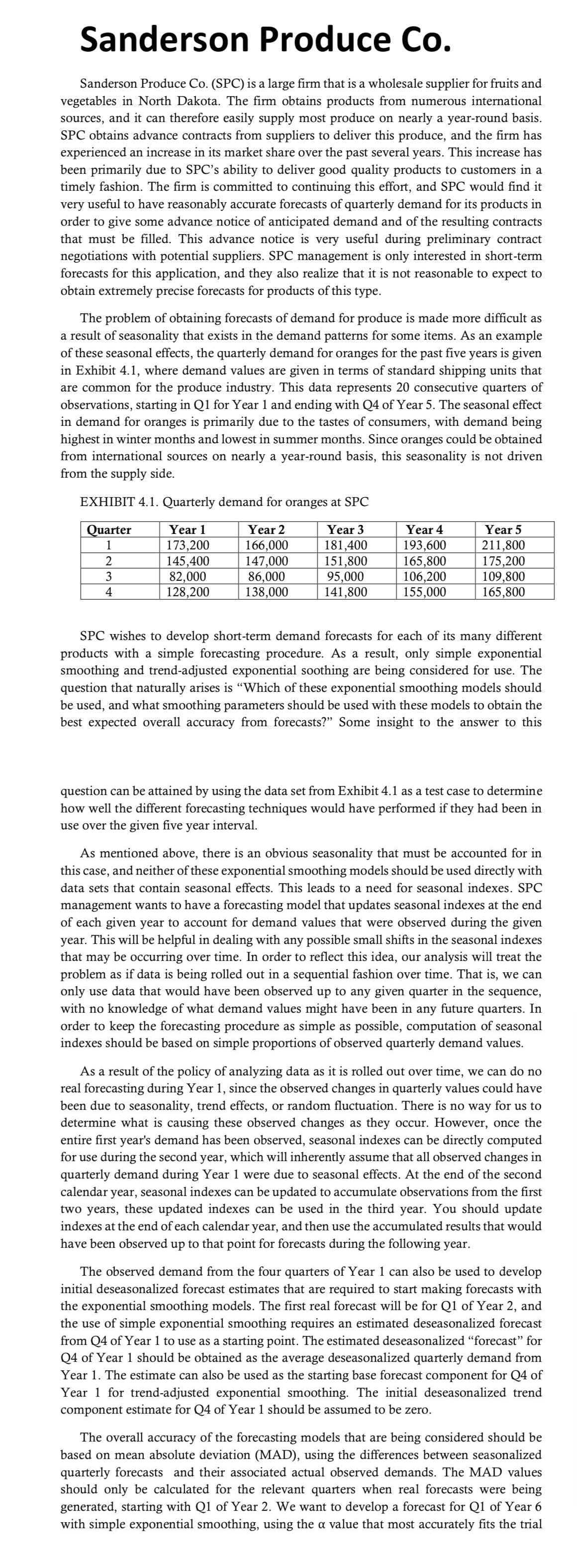SPC management is only interested in short-termforecasts for this application, and they also realize that it is not reasonable to expect toobtain extremely precise forecasts for products of this type.The problem of obtaining forecasts of demand for produce is made more difficult asa result of seasonality that exists in the demand patterns for some items. As an exampleof these seasonal effects, the quarterly demand for oranges for the past five years is givenin Exhibit 4.1, where demand values are given in terms of standard shipping units thatare common for the produce industry. This data represents 20 consecutive quarters ofobservations, starting in Q1 for Year 1 and ending with Q4 of Year 5. The seasonal effectin demand for oranges is primarily due to the tastes of consumers, with demand beinghighest in winter months and lowest in summer months. Since oranges could be obtainedfrom international sources on nearly a year-round basis, this seasonality is not drivenfrom the supply side.EXHIBIT 4.1. Quarterly demand for oranges at SPCQuarterYear 1Year 2Year 31173,200166,000181,4002145,400147,000151,800382,00086,00095,0004128,200138,000141,800Year 4193,600165,800106,200155,000Year 5211,800175,200109,800165,800SPC wishes to develop short-term demand forecasts for each of its many differentproducts with a simple forecasting procedure. As a result, only simple exponentialsmoothing and trend-adjusted exponential soothing are being considered for use. Thequestion that naturally arises is "Which of these exponential smoothing models shouldbe used, and what smoothing parameters should be used with these models to obtain thebest expected overall accuracy from forecasts?" Some insight to the answer to thisquestion can be attained by using the data set from Exhibit 4.1 as a test case to determinehow well the different forecasting techniques would have performed if they had been inuse over the given five year interval.As mentioned above, there is an obvious seasonality that must be accounted for inthis case, and neither of these exponential smoothing models should be used directly withdata sets that contain seasonal effects. This leads to a need for seasonal indexes. SPCmanagement wants to have a forecasting model that updates seasonal indexes at the endof each given year to account for demand values that were observed during the givenyear. This will be helpful in dealing with any possible small shifts in the seasonal indexesthat may be occurring over time. In order to reflect this idea, our analysis will treat theproblem as if data is being rolled out in a sequential fashion over time. That is, we canonly use data that would have been observed up to any given quarter in the sequence,with no knowledge of what demand values might have been in any future quarters. Inorder to keep the forecasting procedure as simple as possible, computation of seasonalindexes should be based on simple proportions of observed quarterly demand values.As a result of the policy of analyzing data as it is rolled out over time, we can do noreal forecasting during Year 1, since the observed changes in quarterly values could havebeen due to seasonality, trend effects, or random fluctuation. There is no way for us todetermine what is causing these observed changes as they occur. However, once theentire first year's demand has been observed, seasonal indexes can be directly computedfor use during the second year, which will inherently assume that all observed changes inquarterly demand during Year 1 were due to seasonal effects. At the end of the secondcalendar year, seasonal indexes can be updated to accumulate observations from the firsttwo years, these updated indexes can be used in the third year. You should updateindexes at the end of each calendar year, and then use the accumulated results that wouldhave been observed up to that point for forecasts during the following year.The observed demand from the four quarters of Year 1 can also be used to developinitial deseasonalized forecast estimates that are required to start making forecasts withthe exponential smoothing models. The first real forecast will be for Q1 of Year 2, andthe use of simple exponential smoothing requires an estimated deseasonalized forecastfrom Q4 of Year 1 to use as a starting point. The estimated deseasonalized "forecast" forQ4 of Year 1 should be obtained as the average deseasonalized quarterly demand fromYear 1. The estimate can also be used as the starting base forecast component for Q4 ofYear 1 for trend-adjusted exponential smoothing. The initial deseasonalized trendcomponent estimate for Q4 of Year 1 should be assumed to be zero.The overall accuracy of the forecasting models that are being considered should bebased on mean absolute deviation (MAD), using the differences between seasonalizedquarterly forecasts and their associated actual observed demands. The MAD valuesshould only be calculated for the relevant quarters when real forecasts were beinggenerated, starting with Q1 of Year 2. We want to develop a forecast for Q1 of Year 6with simple exponential smoothing, using the a value that most accurately fits the trial data set. The tracking signal values that would have been obtained for each quartershould also be computed, with MAD values and tracking signals being calculated as thequarterly demand values are sequentially rolled out. We also want to develop a forecastfor Q1 of Year 6 with trend-adjusted exponential smoothing, using the values of a and 8that most accurately fit the trial data set with trend-adjusted exponential smoothing.Tracking-signal values should also be calculated for each quarter, as they were for thesimple exponential smoothing forecasts. Any observations regarding the efficacy of usingforecasting techniques on the demand data from this particular example, based onobservations from the computed tracking signals, will be of interest to the managementof SPC.The management of SPC has also raised some additional issues regarding theforecasting techniques that might be used. In reality, very different costs are incurred,depending upon whether you over forecast demand or under forecast demand. If youover forecast actual demand for any quarter, you will be contracting to buy more producethan will be required. Some types of surplus produce will have to be discarded as acomplete loss, while other types of produce can be sold at a discount. Some types canonly be sold at significant discount, to be used as food for animals. Other types of producecan be sold to canneries for a less significant discount. If you under forecast, you will notbe able to meet demand, which will result in lost sales, and you will also have someunhappy customers as a result. Such an outcome would be in sharp contrast with thecompany's commitment to meeting the needs of customers, as discussed above. However,the high cost of routinely discarding or discounting surplus produce would be prohibitivefor SPC to absorb on a long term basis.Given all this information, the use of the standard measures of "accuracy" of overallforecast error might be called into question. The SPC management estimates that thepenalty cost for overcasting should be assessed as roughly six times as much per unit offorecast error as the penalty cost for under forecasting. They are interested in having someinsight on the significance of the impact that this relative cost consideration might haveon standard forecasting techniques, relative to the results that were found above. Thisimpact can be shown by developing a quarterly forecast for Q1 of Year 6, with the sameexponential smoothing forecasting model that was considered to be accurate in the firstpart of this study. However, the parameters for the "most accurate" forecasting model inthis situation should be determined on the basis of trying to minimize the total overallcost of forecasting error.**Technical note: If you use the Solver option in Excel to search for the specific a and 8 that minimizeMAD, be careful to use multiple starting points in the a and 8 cells at the start of the search to avoid thepossibility of obtaining "local minimum" solutions for MAD.

Find the Given details below: Given details: Year Quarter Demand 1 1 173200 2 145400 3…

The observed demand from the four quarters of Year 1 can also be used to develop initial deseasonalized forecast estimates that are required to start making forecasts with the exponential smoothing models. The first real forecast will be for Q1 of Year 2, and the use of simple exponential smoothing requires an estimated deseasonalized forecast from Q4 of Year 1 to use as a starting point. The estimated deseasonalized “forecast” for Q4 of Year 1 should be obtained as the average deseasonalized quarterly demand from Year 1. The estimate can also be used as the starting base forecast component for Q4 of Year 1 for trend-adjusted exponential smoothing. The initial deseasonalized trend component estimate for Q4 of Year 1 should be assumed to be zero.

The observed demand from the four quarters of Year 1 can also be used to develop initial deseasonalized forecast estimates that are required to start making forecasts with the exponential smoothing models. The first real forecast will be for Q1 of Year 2, and the use of simple exponential smoothing requires an estimated deseasonalized forecast from Q4 of Year 1 to use as a starting point. The estimated deseasonalized “forecast” for Q4 of Year 1 should be obtained as the average deseasonalized quarterly demand from Year 1. The estimate can also be used as the starting base forecast component for Q4 of Year 1 for trend-adjusted exponential smoothing. The initial deseasonalized trend component estimate for Q4 of Year 1 should be assumed to be zero.

Practical Management Science

6th Edition

ISBN:9781337406659

Author:WINSTON, Wayne L.

Publisher:WINSTON, Wayne L.

Chapter9: Decision Making Under Uncertainty

Section: Chapter Questions

Problem 30P

See similar textbooks

Similar questions

Scenario 3 Ben Gibson, the purchasing manager at Coastal Products, was reviewing purchasing expenditures for packaging materials with Jeff Joyner. Ben was particularly disturbed about the amount spent on corrugated boxes purchased from Southeastern Corrugated. Ben said, I dont like the salesman from that company. He comes around here acting like he owns the place. He loves to tell us about his fancy car, house, and vacations. It seems to me he must be making too much money off of us! Jeff responded that he heard Southeastern Corrugated was going to ask for a price increase to cover the rising costs of raw material paper stock. Jeff further stated that Southeastern would probably ask for more than what was justified simply from rising paper stock costs. After the meeting, Ben decided he had heard enough. After all, he prided himself on being a results-oriented manager. There was no way he was going to allow that salesman to keep taking advantage of Coastal Products. Ben called Jeff and told him it was time to rebid the corrugated contract before Southeastern came in with a price increase request. Who did Jeff know that might be interested in the business? Jeff replied he had several companies in mind to include in the bidding process. These companies would surely come in at a lower price, partly because they used lower-grade boxes that would probably work well enough in Coastal Products process. Jeff also explained that these suppliers were not serious contenders for the business. Their purpose was to create competition with the bids. Ben told Jeff to make sure that Southeastern was well aware that these new suppliers were bidding on the contract. He also said to make sure the suppliers knew that price was going to be the determining factor in this quote, because he considered corrugated boxes to be a standard industry item. As the Marketing Manager for Southeastern Corrugated, what would you do upon receiving the request for quotation from Coastal Products?
The Global Sourcing Wire Harness Decision Sheila Austin, a buyer at Autolink, a Detroit-based producer of subassemblies for the automotive market, has sent out requests for quotations for a wiring harness to four prospective suppliers. Only two of the four suppliers indicated an interest in quoting the business: Original Wire (Auburn Hills, MI) and Happy Lucky Assemblies (HLA) of Guangdong Province, China. The estimated demand for the harnesses is 5,000 units a month. Both suppliers will incur some costs to retool for this particular harness. The harnesses will be prepackaged in 24 12 6-inch cartons. Each packaged unit weighs approximately 10 pounds. Quote 1 The first quote received is from Original Wire. Auburn Hills is about 20 miles from Autolinks corporate headquarters, so the quote was delivered in person. When Sheila went down to the lobby, she was greeted by the sales agent and an engineering representative. After the quote was handed over, the sales agent noted that engineering would be happy to work closely with Autolink in developing the unit and would also be interested in future business that might involve finding ways to reduce costs. The sales agent also noted that they were hungry for business, as they were losing a lot of customers to companies from China. The quote included unit price, tooling, and packaging. The quoted unit price does not include shipping costs. Original Wire requires no special warehousing of inventory, and daily deliveries from its manufacturing site directly to Autolinks assembly operations are possible. Original Wire Quote: Unit price = 30 Packing costs = 0.75 per unit Tooling = 6,000 one-time fixed charge Freight cost = 5.20 per hundred pounds Quote 2 The second quote received is from Happy Lucky Assemblies of Guangdong Province, China. The supplier must pack the harnesses in a container and ship via inland transportation to the port of Shanghai in China, have the shipment transferred to a container ship, ship material to Seattle, and then have material transported inland to Detroit. The quoted unit price does not include international shipping costs, which the buyer will assume. HLA Quote: Unit price = 19.50 Shipping lead time = Eight weeks Tooling = 3,000 In addition to the suppliers quote, Sheila must consider additional costs and information before preparing a comparison of the Chinese suppliers quotation: Each monthly shipment requires three 40-foot containers. Packing costs for containerization = 2 per unit. Cost of inland transportation to port of export = 200 per container. Freight forwarders fee = 100 per shipment (letter of credit, documentation, etc.). Cost of ocean transport = 4,000 per container. This has risen significantly in recent years due to a shortage of ocean freight capacity. Marine insurance = 0.50 per 100 of shipment. U.S. port handling charges = 1,200 per container. This fee has also risen considerably this year, due to increased security. Ports have also been complaining that the charges may increase in the future. Customs duty = 5% of unit cost. Customs broker fees per shipment = 300. Transportation from Seattle to Detroit = 18.60 per hundred pounds. Need to warehouse at least four weeks of inventory in Detroit at a warehousing cost of 1.00 per cubic foot per month, to compensate for lead time uncertainty. Sheila must also figure the costs associated with committing corporate capital for holding inventory. She has spoken to some accountants, who typically use a corporate cost of capital rate of 15%. Cost of hedging currencybroker fees = 400 per shipment Additional administrative time due to international shipping = 4 hours per shipment 25 per hour (estimated) At least two five-day visits per year to travel to China to meet with supplier and provide updates on performance and shipping = 20,000 per year (estimated) The international sourcing costs must be absorbed by Sheila, as the supplier does not assume any of the additional estimated costs and invoice Sheila later, or build the costs into a revised unit price. Sheila feels that the U.S. supplier is probably less expensive, even though it quoted a higher price. Sheila also knows that this is a standard technology that is unlikely to change during the next three years, but which could be a contract that extends multiple years out. There is also a lot of hall talk amongst the engineers on her floor about next-generation automotive electronics, which will completely eliminate the need for wire harnesses, which will be replaced by electronic components that are smaller, lighter, and more reliable. She is unsure about how to calculate the total costs for each option, and she is even more unsure about how to factor these other variables into the decision. Based on this case, do you think international purchasing is more or less complex than domestic purchasing? Why? Is it worth the additional effort?
The Global Sourcing Wire Harness Decision Sheila Austin, a buyer at Autolink, a Detroit-based producer of subassemblies for the automotive market, has sent out requests for quotations for a wiring harness to four prospective suppliers. Only two of the four suppliers indicated an interest in quoting the business: Original Wire (Auburn Hills, MI) and Happy Lucky Assemblies (HLA) of Guangdong Province, China. The estimated demand for the harnesses is 5,000 units a month. Both suppliers will incur some costs to retool for this particular harness. The harnesses will be prepackaged in 24 12 6-inch cartons. Each packaged unit weighs approximately 10 pounds. Quote 1 The first quote received is from Original Wire. Auburn Hills is about 20 miles from Autolinks corporate headquarters, so the quote was delivered in person. When Sheila went down to the lobby, she was greeted by the sales agent and an engineering representative. After the quote was handed over, the sales agent noted that engineering would be happy to work closely with Autolink in developing the unit and would also be interested in future business that might involve finding ways to reduce costs. The sales agent also noted that they were hungry for business, as they were losing a lot of customers to companies from China. The quote included unit price, tooling, and packaging. The quoted unit price does not include shipping costs. Original Wire requires no special warehousing of inventory, and daily deliveries from its manufacturing site directly to Autolinks assembly operations are possible. Original Wire Quote: Unit price = 30 Packing costs = 0.75 per unit Tooling = 6,000 one-time fixed charge Freight cost = 5.20 per hundred pounds Quote 2 The second quote received is from Happy Lucky Assemblies of Guangdong Province, China. The supplier must pack the harnesses in a container and ship via inland transportation to the port of Shanghai in China, have the shipment transferred to a container ship, ship material to Seattle, and then have material transported inland to Detroit. The quoted unit price does not include international shipping costs, which the buyer will assume. HLA Quote: Unit price = 19.50 Shipping lead time = Eight weeks Tooling = 3,000 In addition to the suppliers quote, Sheila must consider additional costs and information before preparing a comparison of the Chinese suppliers quotation: Each monthly shipment requires three 40-foot containers. Packing costs for containerization = 2 per unit. Cost of inland transportation to port of export = 200 per container. Freight forwarders fee = 100 per shipment (letter of credit, documentation, etc.). Cost of ocean transport = 4,000 per container. This has risen significantly in recent years due to a shortage of ocean freight capacity. Marine insurance = 0.50 per 100 of shipment. U.S. port handling charges = 1,200 per container. This fee has also risen considerably this year, due to increased security. Ports have also been complaining that the charges may increase in the future. Customs duty = 5% of unit cost. Customs broker fees per shipment = 300. Transportation from Seattle to Detroit = 18.60 per hundred pounds. Need to warehouse at least four weeks of inventory in Detroit at a warehousing cost of 1.00 per cubic foot per month, to compensate for lead time uncertainty. Sheila must also figure the costs associated with committing corporate capital for holding inventory. She has spoken to some accountants, who typically use a corporate cost of capital rate of 15%. Cost of hedging currencybroker fees = 400 per shipment Additional administrative time due to international shipping = 4 hours per shipment 25 per hour (estimated) At least two five-day visits per year to travel to China to meet with supplier and provide updates on performance and shipping = 20,000 per year (estimated) The international sourcing costs must be absorbed by Sheila, as the supplier does not assume any of the additional estimated costs and invoice Sheila later, or build the costs into a revised unit price. Sheila feels that the U.S. supplier is probably less expensive, even though it quoted a higher price. Sheila also knows that this is a standard technology that is unlikely to change during the next three years, but which could be a contract that extends multiple years out. There is also a lot of hall talk amongst the engineers on her floor about next-generation automotive electronics, which will completely eliminate the need for wire harnesses, which will be replaced by electronic components that are smaller, lighter, and more reliable. She is unsure about how to calculate the total costs for each option, and she is even more unsure about how to factor these other variables into the decision. Calculate the total cost per unit of purchasing from Original Wire.
The Global Sourcing Wire Harness Decision Sheila Austin, a buyer at Autolink, a Detroit-based producer of subassemblies for the automotive market, has sent out requests for quotations for a wiring harness to four prospective suppliers. Only two of the four suppliers indicated an interest in quoting the business: Original Wire (Auburn Hills, MI) and Happy Lucky Assemblies (HLA) of Guangdong Province, China. The estimated demand for the harnesses is 5,000 units a month. Both suppliers will incur some costs to retool for this particular harness. The harnesses will be prepackaged in 24 12 6-inch cartons. Each packaged unit weighs approximately 10 pounds. Quote 1 The first quote received is from Original Wire. Auburn Hills is about 20 miles from Autolinks corporate headquarters, so the quote was delivered in person. When Sheila went down to the lobby, she was greeted by the sales agent and an engineering representative. After the quote was handed over, the sales agent noted that engineering would be happy to work closely with Autolink in developing the unit and would also be interested in future business that might involve finding ways to reduce costs. The sales agent also noted that they were hungry for business, as they were losing a lot of customers to companies from China. The quote included unit price, tooling, and packaging. The quoted unit price does not include shipping costs. Original Wire requires no special warehousing of inventory, and daily deliveries from its manufacturing site directly to Autolinks assembly operations are possible. Original Wire Quote: Unit price = 30 Packing costs = 0.75 per unit Tooling = 6,000 one-time fixed charge Freight cost = 5.20 per hundred pounds Quote 2 The second quote received is from Happy Lucky Assemblies of Guangdong Province, China. The supplier must pack the harnesses in a container and ship via inland transportation to the port of Shanghai in China, have the shipment transferred to a container ship, ship material to Seattle, and then have material transported inland to Detroit. The quoted unit price does not include international shipping costs, which the buyer will assume. HLA Quote: Unit price = 19.50 Shipping lead time = Eight weeks Tooling = 3,000 In addition to the suppliers quote, Sheila must consider additional costs and information before preparing a comparison of the Chinese suppliers quotation: Each monthly shipment requires three 40-foot containers. Packing costs for containerization = 2 per unit. Cost of inland transportation to port of export = 200 per container. Freight forwarders fee = 100 per shipment (letter of credit, documentation, etc.). Cost of ocean transport = 4,000 per container. This has risen significantly in recent years due to a shortage of ocean freight capacity. Marine insurance = 0.50 per 100 of shipment. U.S. port handling charges = 1,200 per container. This fee has also risen considerably this year, due to increased security. Ports have also been complaining that the charges may increase in the future. Customs duty = 5% of unit cost. Customs broker fees per shipment = 300. Transportation from Seattle to Detroit = 18.60 per hundred pounds. Need to warehouse at least four weeks of inventory in Detroit at a warehousing cost of 1.00 per cubic foot per month, to compensate for lead time uncertainty. Sheila must also figure the costs associated with committing corporate capital for holding inventory. She has spoken to some accountants, who typically use a corporate cost of capital rate of 15%. Cost of hedging currencybroker fees = 400 per shipment Additional administrative time due to international shipping = 4 hours per shipment 25 per hour (estimated) At least two five-day visits per year to travel to China to meet with supplier and provide updates on performance and shipping = 20,000 per year (estimated) The international sourcing costs must be absorbed by Sheila, as the supplier does not assume any of the additional estimated costs and invoice Sheila later, or build the costs into a revised unit price. Sheila feels that the U.S. supplier is probably less expensive, even though it quoted a higher price. Sheila also knows that this is a standard technology that is unlikely to change during the next three years, but which could be a contract that extends multiple years out. There is also a lot of hall talk amongst the engineers on her floor about next-generation automotive electronics, which will completely eliminate the need for wire harnesses, which will be replaced by electronic components that are smaller, lighter, and more reliable. She is unsure about how to calculate the total costs for each option, and she is even more unsure about how to factor these other variables into the decision. Based on the total cost per unit, which supplier should Sheila recommend?
The Global Sourcing Wire Harness Decision Sheila Austin, a buyer at Autolink, a Detroit-based producer of subassemblies for the automotive market, has sent out requests for quotations for a wiring harness to four prospective suppliers. Only two of the four suppliers indicated an interest in quoting the business: Original Wire (Auburn Hills, MI) and Happy Lucky Assemblies (HLA) of Guangdong Province, China. The estimated demand for the harnesses is 5,000 units a month. Both suppliers will incur some costs to retool for this particular harness. The harnesses will be prepackaged in 24 12 6-inch cartons. Each packaged unit weighs approximately 10 pounds. Quote 1 The first quote received is from Original Wire. Auburn Hills is about 20 miles from Autolinks corporate headquarters, so the quote was delivered in person. When Sheila went down to the lobby, she was greeted by the sales agent and an engineering representative. After the quote was handed over, the sales agent noted that engineering would be happy to work closely with Autolink in developing the unit and would also be interested in future business that might involve finding ways to reduce costs. The sales agent also noted that they were hungry for business, as they were losing a lot of customers to companies from China. The quote included unit price, tooling, and packaging. The quoted unit price does not include shipping costs. Original Wire requires no special warehousing of inventory, and daily deliveries from its manufacturing site directly to Autolinks assembly operations are possible. Original Wire Quote: Unit price = 30 Packing costs = 0.75 per unit Tooling = 6,000 one-time fixed charge Freight cost = 5.20 per hundred pounds Quote 2 The second quote received is from Happy Lucky Assemblies of Guangdong Province, China. The supplier must pack the harnesses in a container and ship via inland transportation to the port of Shanghai in China, have the shipment transferred to a container ship, ship material to Seattle, and then have material transported inland to Detroit. The quoted unit price does not include international shipping costs, which the buyer will assume. HLA Quote: Unit price = 19.50 Shipping lead time = Eight weeks Tooling = 3,000 In addition to the suppliers quote, Sheila must consider additional costs and information before preparing a comparison of the Chinese suppliers quotation: Each monthly shipment requires three 40-foot containers. Packing costs for containerization = 2 per unit. Cost of inland transportation to port of export = 200 per container. Freight forwarders fee = 100 per shipment (letter of credit, documentation, etc.). Cost of ocean transport = 4,000 per container. This has risen significantly in recent years due to a shortage of ocean freight capacity. Marine insurance = 0.50 per 100 of shipment. U.S. port handling charges = 1,200 per container. This fee has also risen considerably this year, due to increased security. Ports have also been complaining that the charges may increase in the future. Customs duty = 5% of unit cost. Customs broker fees per shipment = 300. Transportation from Seattle to Detroit = 18.60 per hundred pounds. Need to warehouse at least four weeks of inventory in Detroit at a warehousing cost of 1.00 per cubic foot per month, to compensate for lead time uncertainty. Sheila must also figure the costs associated with committing corporate capital for holding inventory. She has spoken to some accountants, who typically use a corporate cost of capital rate of 15%. Cost of hedging currencybroker fees = 400 per shipment Additional administrative time due to international shipping = 4 hours per shipment 25 per hour (estimated) At least two five-day visits per year to travel to China to meet with supplier and provide updates on performance and shipping = 20,000 per year (estimated) The international sourcing costs must be absorbed by Sheila, as the supplier does not assume any of the additional estimated costs and invoice Sheila later, or build the costs into a revised unit price. Sheila feels that the U.S. supplier is probably less expensive, even though it quoted a higher price. Sheila also knows that this is a standard technology that is unlikely to change during the next three years, but which could be a contract that extends multiple years out. There is also a lot of hall talk amongst the engineers on her floor about next-generation automotive electronics, which will completely eliminate the need for wire harnesses, which will be replaced by electronic components that are smaller, lighter, and more reliable. She is unsure about how to calculate the total costs for each option, and she is even more unsure about how to factor these other variables into the decision. Calculate the total cost per unit of purchasing from Happy Lucky Assemblies.
The Global Sourcing Wire Harness Decision Sheila Austin, a buyer at Autolink, a Detroit-based producer of subassemblies for the automotive market, has sent out requests for quotations for a wiring harness to four prospective suppliers. Only two of the four suppliers indicated an interest in quoting the business: Original Wire (Auburn Hills, MI) and Happy Lucky Assemblies (HLA) of Guangdong Province, China. The estimated demand for the harnesses is 5,000 units a month. Both suppliers will incur some costs to retool for this particular harness. The harnesses will be prepackaged in 24 12 6-inch cartons. Each packaged unit weighs approximately 10 pounds. Quote 1 The first quote received is from Original Wire. Auburn Hills is about 20 miles from Autolinks corporate headquarters, so the quote was delivered in person. When Sheila went down to the lobby, she was greeted by the sales agent and an engineering representative. After the quote was handed over, the sales agent noted that engineering would be happy to work closely with Autolink in developing the unit and would also be interested in future business that might involve finding ways to reduce costs. The sales agent also noted that they were hungry for business, as they were losing a lot of customers to companies from China. The quote included unit price, tooling, and packaging. The quoted unit price does not include shipping costs. Original Wire requires no special warehousing of inventory, and daily deliveries from its manufacturing site directly to Autolinks assembly operations are possible. Original Wire Quote: Unit price = 30 Packing costs = 0.75 per unit Tooling = 6,000 one-time fixed charge Freight cost = 5.20 per hundred pounds Quote 2 The second quote received is from Happy Lucky Assemblies of Guangdong Province, China. The supplier must pack the harnesses in a container and ship via inland transportation to the port of Shanghai in China, have the shipment transferred to a container ship, ship material to Seattle, and then have material transported inland to Detroit. The quoted unit price does not include international shipping costs, which the buyer will assume. HLA Quote: Unit price = 19.50 Shipping lead time = Eight weeks Tooling = 3,000 In addition to the suppliers quote, Sheila must consider additional costs and information before preparing a comparison of the Chinese suppliers quotation: Each monthly shipment requires three 40-foot containers. Packing costs for containerization = 2 per unit. Cost of inland transportation to port of export = 200 per container. Freight forwarders fee = 100 per shipment (letter of credit, documentation, etc.). Cost of ocean transport = 4,000 per container. This has risen significantly in recent years due to a shortage of ocean freight capacity. Marine insurance = 0.50 per 100 of shipment. U.S. port handling charges = 1,200 per container. This fee has also risen considerably this year, due to increased security. Ports have also been complaining that the charges may increase in the future. Customs duty = 5% of unit cost. Customs broker fees per shipment = 300. Transportation from Seattle to Detroit = 18.60 per hundred pounds. Need to warehouse at least four weeks of inventory in Detroit at a warehousing cost of 1.00 per cubic foot per month, to compensate for lead time uncertainty. Sheila must also figure the costs associated with committing corporate capital for holding inventory. She has spoken to some accountants, who typically use a corporate cost of capital rate of 15%. Cost of hedging currencybroker fees = 400 per shipment Additional administrative time due to international shipping = 4 hours per shipment 25 per hour (estimated) At least two five-day visits per year to travel to China to meet with supplier and provide updates on performance and shipping = 20,000 per year (estimated) The international sourcing costs must be absorbed by Sheila, as the supplier does not assume any of the additional estimated costs and invoice Sheila later, or build the costs into a revised unit price. Sheila feels that the U.S. supplier is probably less expensive, even though it quoted a higher price. Sheila also knows that this is a standard technology that is unlikely to change during the next three years, but which could be a contract that extends multiple years out. There is also a lot of hall talk amongst the engineers on her floor about next-generation automotive electronics, which will completely eliminate the need for wire harnesses, which will be replaced by electronic components that are smaller, lighter, and more reliable. She is unsure about how to calculate the total costs for each option, and she is even more unsure about how to factor these other variables into the decision. Are there any other issues besides cost that Sheila should evaluate?
Scenario 4 Sharon Gillespie, a new buyer at Visionex, Inc., was reviewing quotations for a tooling contract submitted by four suppliers. She was evaluating the quotes based on price, target quality levels, and delivery lead time promises. As she was working, her manager, Dave Cox, entered her office. He asked how everything was progressing and if she needed any help. She mentioned she was reviewing quotations from suppliers for a tooling contract. Dave asked who the interested suppliers were and if she had made a decision. Sharon indicated that one supplier, Apex, appeared to fit exactly the requirements Visionex had specified in the proposal. Dave told her to keep up the good work. Later that day Dave again visited Sharons office. He stated that he had done some research on the suppliers and felt that another supplier, Micron, appeared to have the best track record with Visionex. He pointed out that Sharons first choice was a new supplier to Visionex and there was some risk involved with that choice. Dave indicated that it would please him greatly if she selected Micron for the contract. The next day Sharon was having lunch with another buyer, Mark Smith. She mentioned the conversation with Dave and said she honestly felt that Apex was the best choice. When Mark asked Sharon who Dave preferred, she answered, Micron. At that point Mark rolled his eyes and shook his head. Sharon asked what the body language was all about. Mark replied, Look, I know youre new but you should know this. I heard last week that Daves brother-in-law is a new part owner of Micron. I was wondering how soon it would be before he started steering business to that company. He is not the straightest character. Sharon was shocked. After a few moments, she announced that her original choice was still the best selection. At that point Mark reminded Sharon that she was replacing a terminated buyer who did not go along with one of Daves previous preferred suppliers. Ethical decisions that affect a buyers ethical perspective usually involve the organizational environment, cultural environment, personal environment, and industry environment. Analyze this scenario using these four variables.
Scenario 4 Sharon Gillespie, a new buyer at Visionex, Inc., was reviewing quotations for a tooling contract submitted by four suppliers. She was evaluating the quotes based on price, target quality levels, and delivery lead time promises. As she was working, her manager, Dave Cox, entered her office. He asked how everything was progressing and if she needed any help. She mentioned she was reviewing quotations from suppliers for a tooling contract. Dave asked who the interested suppliers were and if she had made a decision. Sharon indicated that one supplier, Apex, appeared to fit exactly the requirements Visionex had specified in the proposal. Dave told her to keep up the good work. Later that day Dave again visited Sharons office. He stated that he had done some research on the suppliers and felt that another supplier, Micron, appeared to have the best track record with Visionex. He pointed out that Sharons first choice was a new supplier to Visionex and there was some risk involved with that choice. Dave indicated that it would please him greatly if she selected Micron for the contract. The next day Sharon was having lunch with another buyer, Mark Smith. She mentioned the conversation with Dave and said she honestly felt that Apex was the best choice. When Mark asked Sharon who Dave preferred, she answered, Micron. At that point Mark rolled his eyes and shook his head. Sharon asked what the body language was all about. Mark replied, Look, I know youre new but you should know this. I heard last week that Daves brother-in-law is a new part owner of Micron. I was wondering how soon it would be before he started steering business to that company. He is not the straightest character. Sharon was shocked. After a few moments, she announced that her original choice was still the best selection. At that point Mark reminded Sharon that she was replacing a terminated buyer who did not go along with one of Daves previous preferred suppliers. What should Sharon do in this situation?
Scenario 4 Sharon Gillespie, a new buyer at Visionex, Inc., was reviewing quotations for a tooling contract submitted by four suppliers. She was evaluating the quotes based on price, target quality levels, and delivery lead time promises. As she was working, her manager, Dave Cox, entered her office. He asked how everything was progressing and if she needed any help. She mentioned she was reviewing quotations from suppliers for a tooling contract. Dave asked who the interested suppliers were and if she had made a decision. Sharon indicated that one supplier, Apex, appeared to fit exactly the requirements Visionex had specified in the proposal. Dave told her to keep up the good work. Later that day Dave again visited Sharons office. He stated that he had done some research on the suppliers and felt that another supplier, Micron, appeared to have the best track record with Visionex. He pointed out that Sharons first choice was a new supplier to Visionex and there was some risk involved with that choice. Dave indicated that it would please him greatly if she selected Micron for the contract. The next day Sharon was having lunch with another buyer, Mark Smith. She mentioned the conversation with Dave and said she honestly felt that Apex was the best choice. When Mark asked Sharon who Dave preferred, she answered, Micron. At that point Mark rolled his eyes and shook his head. Sharon asked what the body language was all about. Mark replied, Look, I know youre new but you should know this. I heard last week that Daves brother-in-law is a new part owner of Micron. I was wondering how soon it would be before he started steering business to that company. He is not the straightest character. Sharon was shocked. After a few moments, she announced that her original choice was still the best selection. At that point Mark reminded Sharon that she was replacing a terminated buyer who did not go along with one of Daves previous preferred suppliers. What does the Institute of Supply Management code of ethics say about financial conflicts of interest?
Avion, Inc. Susan Dey and Bill Mifflin, procurement managers at Avion, Inc., sat across from each other and reviewed a troubling performance report concerning a key supplier, Foster Technologies. The report detailed the deteriorating performance of Foster Technologies in the areas of material quality and on-time delivery. At this point, Kevin ODonnell, another procurement manager, entered the room. Explain the role of performance measurement in managing supply chain activities.
Problem 4-11 (Algorithmic) Edwards Manufacturing Company purchases two component parts from three different suppliers. The suppliers have limited capacity, and no one supplier can meet all the company’s needs. In addition, the suppliers charge different prices for the components. Component price data (in price per unit) are as follows: Supplier Component 1 2 3 1 $11 $12 $13 2 $9 $10 $9 Each supplier has a limited capacity in terms of the total number of components it can supply. However, as long as Edwards provides sufficient advance orders, each supplier can devote its capacity to component 1, component 2, or any combination of the two components, if the total number of units ordered is within its capacity. Supplier capacities are as follows: Supplier 1 2 3 Capacity 500 900 700 If the Edwards production plan for the next period includes 900 units of component 1 and 700 units of component 2, what purchases do you recommend? That is, how many units of each…
DM Office Products (DMOP) is a wholesale supplier of office products with one facility in Pennsylvania. It has decided to build a new distribution warehouse in the state of New York to help serve the growing demand in that market. It has four major customers located in Buffalo, Syracuse, Albany, and New York City. Though New York City is the largest market, it also has the greatest competition, and DMOP is not a major player there. When DMOP ships an order to a customer, it uses its own small fleet of two trucks to deliver, so the cost of delivery is essentially the same for a full or partially full truck. The expected number of annual shipments to each city and their coordinates on an x, y grid is shown in the following table. CITY x-COORDINATES y-COORDINATES NUMBER OF SHIPMENTS Buffalo 340 865 85 Syracuse 1,435 915 89 Albany 2,315 645 129 New York City 2,290 45 69