This homework deals with applications of concepts related to the Bilateral Laplace Transform, or otherwise known as the BLT 1. For the circuit shown, the voltage source x(t) is the input and the current y(t) y(t) is the output. Write the differential equation of the cireuit relating the input L and the output without assigning x(t) numerical values to the eireuit elements 2. Use the differential equation developed in Prob. 1 to obtain the transfer function H(s) of the system (circuit) 3. Assume now for simplicity that the circuit elements have the unrealistic values of 10 1H, and 1F. Draw the pole-zero plot of the transfer function of the system using these component values. 4. Use graphical methods to evaluate and plot the magnitude of the transfer function H(j@) as a function of o. Show five separate pole-zero plots and the associated vectors. One plot will be done with o=0 rps, the next one with o=0.5 rps , the next one with o-1rps, the next one with -5 rps , and the last one with o->rps. Determine the length of the veetors for each frequency value and use those to estimate the value of | H(jø)| at each of the frequencies. Use those values to plot the magnitude of the transfer function and determine what kind of filter the system implements. This problem must be done by hand. You can use MATLAB to confirm the correctness of your results but MATLAB work for this problem will not be accepted and if turned in will receive no credit 5. Use graphical methods to evaluate and plot the phase of the transfer function Hjø) as a function of o. Show five separate pole-zero plots and the associated vectors. One plot will be done with o 0 rps, the next one with o= 0.5 rps , the next one with o -1rps, the next one with -5rps, and the last one with o-» rps. Determine the angles of the vectors for each frequency value and use those to estimate the value of ZH(jø) at each of the frequencies. Plot the points in order to get a phase plot of the transfer function. This problem must be done bv hand. You can use MATLAB to confirm the correctness of vour results but MATLAB work for this problem will not be acceepted and if turned in will receive no credit 6. Assume a system having input x(t) and output y(t) is described by the transfer function Y(s) H(s) with ROC a-a. Write the differential equation of this system X(s) a relating the input and the output. I think you will agree that this looks like a standard first order differential equation you have seen many times. However, given the ROC and the fact that the transfer function and impulse response are transform pairs, the impulse response of this system must be (look at the tables) ht) = -e""u(-t). In other words a unit impulse applied at time t 0 produces a backward (in time) response. Verify that the h(t) is indeed the solution of the differential equation when a unit impulse is applied at r =0. 7. Suppose that the input to the system of Prob. 6 is a regular unit step u(t). Attempt to obtain the output of the system by convolution for the case where a 0. You are likely to run into trouble. Why? Now attempt to use Laplace Transforms to obtain the output. Does this overcome the problem encountered in using convolution? Look at the ROc's of the Laplace Transforms of the two time functions that are being convolved. Does this explain the difficulties encountered in obtaining the output via convolution? Now repeat this process for a < 0. Obtaining the output via convolution should work. What is the output? Looking at the ROCS of the signals being convolved, does this explain why convolution works now while it did not before? 8. Use the BLT to obtain the output of the system of Prob. 6 when the input is xt)eu(-t Consider both cases, a =b and a #b. Do not assign numerical values to these two constants 9. Use MATLAB to plot the result of Prob. 8, in one case for a =b=-3 and in the other case for a -1 and b1 These problems must be worked on independently and tuned in at the beginning of elass on Tuesday Nov. 26, 2019. You are required to place a cover sheet in front of the papers showing your work. The cover sheet to be used is shown on the next page which can be copied directly or can be your own creation using the exact same format shown. Save the cover page for modification and future use as all homework turned in will have to have the cover page with appropriate dates, etc.
This homework deals with applications of concepts related to the Bilateral Laplace Transform, or otherwise known as the BLT 1. For the circuit shown, the voltage source x(t) is the input and the current y(t) y(t) is the output. Write the differential equation of the cireuit relating the input L and the output without assigning x(t) numerical values to the eireuit elements 2. Use the differential equation developed in Prob. 1 to obtain the transfer function H(s) of the system (circuit) 3. Assume now for simplicity that the circuit elements have the unrealistic values of 10 1H, and 1F. Draw the pole-zero plot of the transfer function of the system using these component values. 4. Use graphical methods to evaluate and plot the magnitude of the transfer function H(j@) as a function of o. Show five separate pole-zero plots and the associated vectors. One plot will be done with o=0 rps, the next one with o=0.5 rps , the next one with o-1rps, the next one with -5 rps , and the last one with o->rps. Determine the length of the veetors for each frequency value and use those to estimate the value of | H(jø)| at each of the frequencies. Use those values to plot the magnitude of the transfer function and determine what kind of filter the system implements. This problem must be done by hand. You can use MATLAB to confirm the correctness of your results but MATLAB work for this problem will not be accepted and if turned in will receive no credit 5. Use graphical methods to evaluate and plot the phase of the transfer function Hjø) as a function of o. Show five separate pole-zero plots and the associated vectors. One plot will be done with o 0 rps, the next one with o= 0.5 rps , the next one with o -1rps, the next one with -5rps, and the last one with o-» rps. Determine the angles of the vectors for each frequency value and use those to estimate the value of ZH(jø) at each of the frequencies. Plot the points in order to get a phase plot of the transfer function. This problem must be done bv hand. You can use MATLAB to confirm the correctness of vour results but MATLAB work for this problem will not be acceepted and if turned in will receive no credit 6. Assume a system having input x(t) and output y(t) is described by the transfer function Y(s) H(s) with ROC a-a. Write the differential equation of this system X(s) a relating the input and the output. I think you will agree that this looks like a standard first order differential equation you have seen many times. However, given the ROC and the fact that the transfer function and impulse response are transform pairs, the impulse response of this system must be (look at the tables) ht) = -e""u(-t). In other words a unit impulse applied at time t 0 produces a backward (in time) response. Verify that the h(t) is indeed the solution of the differential equation when a unit impulse is applied at r =0. 7. Suppose that the input to the system of Prob. 6 is a regular unit step u(t). Attempt to obtain the output of the system by convolution for the case where a 0. You are likely to run into trouble. Why? Now attempt to use Laplace Transforms to obtain the output. Does this overcome the problem encountered in using convolution? Look at the ROc's of the Laplace Transforms of the two time functions that are being convolved. Does this explain the difficulties encountered in obtaining the output via convolution? Now repeat this process for a < 0. Obtaining the output via convolution should work. What is the output? Looking at the ROCS of the signals being convolved, does this explain why convolution works now while it did not before? 8. Use the BLT to obtain the output of the system of Prob. 6 when the input is xt)eu(-t Consider both cases, a =b and a #b. Do not assign numerical values to these two constants 9. Use MATLAB to plot the result of Prob. 8, in one case for a =b=-3 and in the other case for a -1 and b1 These problems must be worked on independently and tuned in at the beginning of elass on Tuesday Nov. 26, 2019. You are required to place a cover sheet in front of the papers showing your work. The cover sheet to be used is shown on the next page which can be copied directly or can be your own creation using the exact same format shown. Save the cover page for modification and future use as all homework turned in will have to have the cover page with appropriate dates, etc.

Introductory Circuit Analysis (13th Edition)
13th Edition
ISBN:9780133923605
Author:Robert L. Boylestad
Publisher:Robert L. Boylestad
Chapter1: Introduction
Section: Chapter Questions
Problem 1P: Visit your local library (at school or home) and describe the extent to which it provides literature...

Related questions
Question
Transcribed Image Text:This homework deals with applications of concepts related to the Bilateral Laplace
Transform, or otherwise known as the BLT
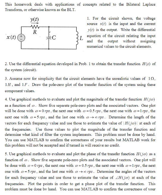
1. For the circuit shown, the voltage
source x(t) is the input and the current
y(t)
y(t) is the output. Write the differential
equation of the cireuit relating the input
L
and the output without assigning
x(t)
numerical values to the eireuit elements
2. Use the differential equation developed in Prob. 1 to obtain the transfer function H(s) of
the system (circuit)
3. Assume now for simplicity that the circuit elements have the unrealistic values of 10
1H, and 1F. Draw the pole-zero plot of the transfer function of the system using these
component values.
4. Use graphical methods to evaluate and plot the magnitude of the transfer function H(j@)
as a function of o. Show five separate pole-zero plots and the associated vectors. One plot
will be done with o=0 rps, the next one with o=0.5 rps , the next one with o-1rps, the
next one with -5 rps , and the last one with o->rps. Determine the length of the
veetors for each frequency value and use those to estimate the value of | H(jø)| at each of
the frequencies. Use those values to plot the magnitude of the transfer function and
determine what kind of filter the system implements. This problem must be done by hand.
You can use MATLAB to confirm the correctness of your results but MATLAB work for
this problem will not be accepted and if turned in will receive no credit
5. Use graphical methods to evaluate and plot the phase of the transfer function Hjø) as a
function of o. Show five separate pole-zero plots and the associated vectors. One plot will
be done with o 0 rps, the next one with o= 0.5 rps , the next one with o -1rps, the next
one with -5rps, and the last one with o-» rps. Determine the angles of the vectors
for each frequency value and use those to estimate the value of ZH(jø) at each of the
frequencies. Plot the points in order to get a phase plot of the transfer function. This
problem must be done bv hand. You can use MATLAB to confirm the correctness of vour
Transcribed Image Text:results but MATLAB work for this problem will not be acceepted and if turned in will receive
no credit
6. Assume a system having input x(t) and output y(t) is described by the transfer function
Y(s)
H(s)
with ROC a-a. Write the differential equation of this system
X(s) a
relating the input and the output. I think you will agree that this looks like a standard first
order differential equation you have seen many times. However, given the ROC and the fact
that the transfer function and impulse response are transform pairs, the impulse response of
this system must be (look at the tables) ht) = -e""u(-t). In other words a unit impulse
applied at time t 0 produces a backward (in time) response. Verify that the h(t) is indeed
the solution of the differential equation when a unit impulse is applied at r =0.
7. Suppose that the input to the system of Prob. 6 is a regular unit step u(t). Attempt to
obtain the output of the system by convolution for the case where a 0. You are likely to
run into trouble. Why? Now attempt to use Laplace Transforms to obtain the output. Does
this overcome the problem encountered in using convolution? Look at the ROc's of the
Laplace Transforms of the two time functions that are being convolved. Does this explain
the difficulties encountered in obtaining the output via convolution? Now repeat this process
for a < 0. Obtaining the output via convolution should work. What is the output? Looking
at the ROCS of the signals being convolved, does this explain why convolution works now
while it did not before?
8. Use the BLT to obtain the output of the system of Prob. 6 when the input is
xt)eu(-t Consider both cases, a =b and a #b. Do not assign numerical values to
these two constants
9. Use MATLAB to plot the result of Prob. 8, in one case for a =b=-3 and in the other case
for a -1 and b1
These problems must be worked on independently and tuned in at the beginning of elass on
Tuesday Nov. 26, 2019. You are required to place a cover sheet in front of the papers
showing your work. The cover sheet to be used is shown on the next page which can be
copied directly or can be your own creation using the exact same format shown. Save the
cover page for modification and future use as all homework turned in will have to have the
cover page with appropriate dates, etc.
Expert Solution
This question has been solved!
Explore an expertly crafted, step-by-step solution for a thorough understanding of key concepts.

This is a popular solution!

Trending now
This is a popular solution!

Step by step
Solved in 5 steps with 4 images

Recommended textbooks for you
Introductory Circuit Analysis (13th Edition)
Electrical Engineering
ISBN:
9780133923605
Author:
Robert L. Boylestad
Publisher:
PEARSON

Delmar's Standard Textbook Of Electricity
Electrical Engineering
ISBN:
9781337900348
Author:
Stephen L. Herman
Publisher:
Cengage Learning

Programmable Logic Controllers
Electrical Engineering
ISBN:
9780073373843
Author:
Frank D. Petruzella
Publisher:
McGraw-Hill Education
Introductory Circuit Analysis (13th Edition)
Electrical Engineering
ISBN:
9780133923605
Author:
Robert L. Boylestad
Publisher:
PEARSON
Delmar's Standard Textbook Of Electricity
Electrical Engineering
ISBN:
9781337900348
Author:
Stephen L. Herman
Publisher:
Cengage Learning
Programmable Logic Controllers
Electrical Engineering
ISBN:
9780073373843
Author:
Frank D. Petruzella
Publisher:
McGraw-Hill Education

Fundamentals of Electric Circuits
Electrical Engineering
ISBN:
9780078028229
Author:
Charles K Alexander, Matthew Sadiku
Publisher:
McGraw-Hill Education

Electric Circuits. (11th Edition)
Electrical Engineering
ISBN:
9780134746968
Author:
James W. Nilsson, Susan Riedel
Publisher:
PEARSON

Engineering Electromagnetics
Electrical Engineering
ISBN:
9780078028151
Author:
Hayt, William H. (william Hart), Jr, BUCK, John A.
Publisher:
Mcgraw-hill Education,