What is the iterative method in system of linear equations? 2. Give atleast two examples of each iterative method. Answer question number 1 only. These is the reference that might help to answer the question.
What is the iterative method in system of linear equations? 2. Give atleast two examples of each iterative method. Answer question number 1 only. These is the reference that might help to answer the question.

Functions and Change: A Modeling Approach to College Algebra (MindTap Course List)
6th Edition
ISBN:9781337111348
Author:Bruce Crauder, Benny Evans, Alan Noell
Publisher:Bruce Crauder, Benny Evans, Alan Noell
Chapter2: Graphical And Tabular Analysis
Section2.3: Solving Linear Equations
Problem 25E

Related questions
Question
1. What is the iterative method in system of linear equations?
2. Give atleast two examples of each iterative method.
Answer question number 1 only.
These is the reference that might help to answer the question.
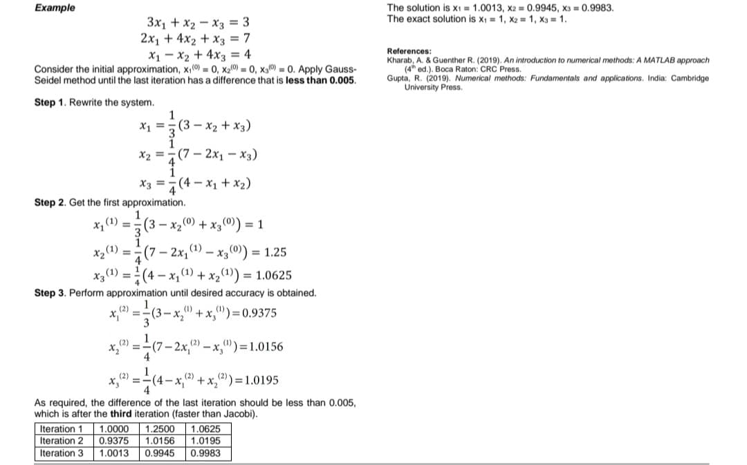
Transcribed Image Text:The solution is X1 = 1.0013, X2 = 0.9945, X3 = 0.9983.
The exact solution is x = 1, X2 = 1, X3 = 1.
Example
3x1 + x2 - x3 = 3
2x1 + 4x2 + x3 = 7
X1 - x2 + 4x3 = 4
Consider the initial approximation, x1(0) = 0, x2(0) = 0, x3) = 0. Apply Gauss-
Seidel method until the last iteration has a difference that is less than 0.005.
References:
Kharab, A. & Guenther R. (2019). An introduction t
(4 ed.). Boca Raton: CRC Press.
Gupta, R. (2019). Numerical methods: Fundamentals and applications. India: Cambridge
University Press,
numerical methods: A MATLAB approach
Step 1. Rewrite the system.
X1 =,(3 – x2 + x3)
x2 = (7 – 2x1 – x3)
x3 = (4 - x1 + x2)
Step 2. Get the first approximation.
x,(1)
=(3 – x2(0) + x3(0)) = 1
X2(1)
=-(7 – 2x,
- x3(0)) = 1.25
x3(1) = (4 – x,(1) + x2(1)) = 1.0625
%3D
Step 3. Perform approximation until desired accuracy is obtained.
1
=-(3-x," + x,"
3
(2)
(") 0.9375
(7–2x,2) – x,"))=1.0156
4
(2) =
(2) -
(2)
(4-x,4 +x,2))= 1.0195
4
As required, the difference of the last iteration should be less than 0.005,
which is after the third iteration (faster than Jacobi).
1.0000
| 1.0625
1.0195
0.9983
Iteration 1
1.2500
Iteration 2
0.9375
1.0156
Iteration 3
1.0013
0.9945
![Systems of Linear Equations (Iterative Methods)
Iterative methods are based on successive improvement of initial guesses
for the solution.
The first approximation [x1(1), x2(1), ..., Xn(1)] is used to solve for the second
iteration. The process is repeated until desired accuracy is obtained. The
(k+1)th iteration can be obtained from kth iteration by the following formula:
x,
(k+1) =b,-(a,x,4) + a,zx,«) +•.+a„x„")]
%3D
Iterative Method 1:
Jacobi Method/Method of
Simultaneous
Displacement
1
x, (k).
(k)
(k) +...+azX
(k+1)
x,
The linear system of equations can be rewritten as:
-[b, - (a,,x, +a3X, +…·+a„X,
(k+1)
%3D
(k).
k = 0,1,2,...
a
1
x, =
-b, - (a,x, +a,x, + +a„X,
The Jacobi iteration formula can be written as:
1
(k+1)
%3D
(k)
1sisn k=0,1,2,...
j=1
X =
-b, - (a,x, +aX2 ++a,n-1\,-1
a
Example
Initial approximation is required to get the next approximation. Let the initial
approximation be [x1©, x2), .., Xn]. These values are used to get the next
approximation [x,("), x2(1), ..., xn")] of the Jacobi method.
3x1 + x2 – x3 = 3
2x1 + 4x2 + x3 = 7
X1 - x2 + 4x3 = 4
(1)
%3D
- b, - (a,,x2 + a,3x, +.+a,„X„")]
(0)
(0)
(0)
Consider the initial approximation, x,0) = 0, x20) = 0, x30) = 0. Apply Jacobi
method until the last iteration has a difference that is less than 0.005.
(1)
(0)
,- (a,x +azx
Step 1. Rewrite the system.
1
X1 = (3 – x2 + x3)
(1)
%3D
x2 = (7 – 2x1 – x3)
(0)
b,-(a,x,® +a„zx," +…+a,n-*n-")|
ann
X3 =7(4 – x1 + x2)
06 Handout 1
E student.feedback@sti.edu
*Property of STI
Page 1 of 3
ASTI
IT1903
Step 2. Get the first approximation.
Solve for the approximation of variable x1:
1
(1)
(0)
(1)
(0)
(0)
(0)
(3-x, +x,'
3
)=1
Co"x"lv+..+ o*xlv)– 'q ]
x,"
(1)
=-(7-2x,0 – x,)=1.75
(0)
To solve for x2(1), use x1(1) instead of x1(0) (as used in Jacobi):
4
1
b,-(a,x," +a,x,
(1)
(0)
(0)
X,
+..+a,„x,") |
x, ),
-(4-x, + x,")=1
4
%3D
(0
Solve for the first approximation to the ith variable:
Step 3. Perform approximation until desired accuracy is obtained.
+a* +.+ax,
%3D
1
(2)
(1)
(3-x,"+x,")=0.75
3
X" =.
The last variable is calculated as:
6, - (a,,x," +a„X
a
(1)
(1)
(1)
+...+a,n-1Xn-1
(2)
(1)
(7-2x," - x,)=1
4
X, =.
The first approximation [x1("), x2"), ..., x,(")] is used to solve for the second
iteration. The (k+1)th iteration can be obtained from kth iteration by the
following formula:
(2)
(1)
x, =.
(4-x,
+x,")=1.1875
As required, the difference of the last iteration should be less than 0.005,
which is after the sixth iteration.
(k) +...+ aX,
%3D
a
Iteration 1
Iteration 2
1.0000 1.7500| 1.0000
1.1875
1.0625
1.0039
0.9896
0.9962
1.0000
1.0625 1.0781
0.7500
-(
Iteration 3
Iteration 4
Iteration 5
0.9948 0.9531
1.0169 1.0016
0.9960 | 0.9941
Iteration 6
(k+1) + a,X2
(k+1) =
*+1) +.+a,x**)) k= 0,1,2,...
(k+1)
The solution is x1 = 0.9960, x2 = 0.9941, X3 = 0.9962.
The exact solution is x1 = 1, X2 = 1, X3 = 1.
a
The Gauss-Seidel iteration formula can be written as:
Iterative Method 2: Gauss-Seidel Method/Method of Successive
1
(k+1)
(k)
1sisn k=0,1,2,..
(k+1)
Displacement/Liebmann Method
a,
j=l
Let the initial approximation be [x,(0), x20), ..., x,]. The latest available
values are used to get the next approximation. Let the next approximation
be (x"), x2"), ..., Xn()].](/v2/_next/image?url=https%3A%2F%2Fcontent.bartleby.com%2Fqna-images%2Fquestion%2Ffe92e190-21eb-4bbd-ab9b-abe2398bf339%2Fa925ab12-b539-4bc6-83ef-921247754266%2F4ne5aqn_processed.jpeg&w=3840&q=75)
Transcribed Image Text:Systems of Linear Equations (Iterative Methods)
Iterative methods are based on successive improvement of initial guesses
for the solution.
The first approximation [x1(1), x2(1), ..., Xn(1)] is used to solve for the second
iteration. The process is repeated until desired accuracy is obtained. The
(k+1)th iteration can be obtained from kth iteration by the following formula:
x,
(k+1) =b,-(a,x,4) + a,zx,«) +•.+a„x„")]
%3D
Iterative Method 1:
Jacobi Method/Method of
Simultaneous
Displacement
1
x, (k).
(k)
(k) +...+azX
(k+1)
x,
The linear system of equations can be rewritten as:
-[b, - (a,,x, +a3X, +…·+a„X,
(k+1)
%3D
(k).
k = 0,1,2,...
a
1
x, =
-b, - (a,x, +a,x, + +a„X,
The Jacobi iteration formula can be written as:
1
(k+1)
%3D
(k)
1sisn k=0,1,2,...
j=1
X =
-b, - (a,x, +aX2 ++a,n-1\,-1
a
Example
Initial approximation is required to get the next approximation. Let the initial
approximation be [x1©, x2), .., Xn]. These values are used to get the next
approximation [x,("), x2(1), ..., xn")] of the Jacobi method.
3x1 + x2 – x3 = 3
2x1 + 4x2 + x3 = 7
X1 - x2 + 4x3 = 4
(1)
%3D
- b, - (a,,x2 + a,3x, +.+a,„X„")]
(0)
(0)
(0)
Consider the initial approximation, x,0) = 0, x20) = 0, x30) = 0. Apply Jacobi
method until the last iteration has a difference that is less than 0.005.
(1)
(0)
,- (a,x +azx
Step 1. Rewrite the system.
1
X1 = (3 – x2 + x3)
(1)
%3D
x2 = (7 – 2x1 – x3)
(0)
b,-(a,x,® +a„zx," +…+a,n-*n-")|
ann
X3 =7(4 – x1 + x2)
06 Handout 1
E student.feedback@sti.edu
*Property of STI
Page 1 of 3
ASTI
IT1903
Step 2. Get the first approximation.
Solve for the approximation of variable x1:
1
(1)
(0)
(1)
(0)
(0)
(0)
(3-x, +x,'
3
)=1
Co"x"lv+..+ o*xlv)– 'q ]
x,"
(1)
=-(7-2x,0 – x,)=1.75
(0)
To solve for x2(1), use x1(1) instead of x1(0) (as used in Jacobi):
4
1
b,-(a,x," +a,x,
(1)
(0)
(0)
X,
+..+a,„x,") |
x, ),
-(4-x, + x,")=1
4
%3D
(0
Solve for the first approximation to the ith variable:
Step 3. Perform approximation until desired accuracy is obtained.
+a* +.+ax,
%3D
1
(2)
(1)
(3-x,"+x,")=0.75
3
X" =.
The last variable is calculated as:
6, - (a,,x," +a„X
a
(1)
(1)
(1)
+...+a,n-1Xn-1
(2)
(1)
(7-2x," - x,)=1
4
X, =.
The first approximation [x1("), x2"), ..., x,(")] is used to solve for the second
iteration. The (k+1)th iteration can be obtained from kth iteration by the
following formula:
(2)
(1)
x, =.
(4-x,
+x,")=1.1875
As required, the difference of the last iteration should be less than 0.005,
which is after the sixth iteration.
(k) +...+ aX,
%3D
a
Iteration 1
Iteration 2
1.0000 1.7500| 1.0000
1.1875
1.0625
1.0039
0.9896
0.9962
1.0000
1.0625 1.0781
0.7500
-(
Iteration 3
Iteration 4
Iteration 5
0.9948 0.9531
1.0169 1.0016
0.9960 | 0.9941
Iteration 6
(k+1) + a,X2
(k+1) =
*+1) +.+a,x**)) k= 0,1,2,...
(k+1)
The solution is x1 = 0.9960, x2 = 0.9941, X3 = 0.9962.
The exact solution is x1 = 1, X2 = 1, X3 = 1.
a
The Gauss-Seidel iteration formula can be written as:
Iterative Method 2: Gauss-Seidel Method/Method of Successive
1
(k+1)
(k)
1sisn k=0,1,2,..
(k+1)
Displacement/Liebmann Method
a,
j=l
Let the initial approximation be [x,(0), x20), ..., x,]. The latest available
values are used to get the next approximation. Let the next approximation
be (x"), x2"), ..., Xn()].
Expert Solution
This question has been solved!
Explore an expertly crafted, step-by-step solution for a thorough understanding of key concepts.

Step by step
Solved in 2 steps with 4 images

Recommended textbooks for you
Functions and Change: A Modeling Approach to Coll…
Algebra
ISBN:
9781337111348
Author:
Bruce Crauder, Benny Evans, Alan Noell
Publisher:
Cengage Learning


Algebra & Trigonometry with Analytic Geometry
Algebra
ISBN:
9781133382119
Author:
Swokowski
Publisher:
Cengage
Functions and Change: A Modeling Approach to Coll…
Algebra
ISBN:
9781337111348
Author:
Bruce Crauder, Benny Evans, Alan Noell
Publisher:
Cengage Learning
Algebra & Trigonometry with Analytic Geometry
Algebra
ISBN:
9781133382119
Author:
Swokowski
Publisher:
Cengage

Linear Algebra: A Modern Introduction
Algebra
ISBN:
9781285463247
Author:
David Poole
Publisher:
Cengage Learning

College Algebra
Algebra
ISBN:
9781305115545
Author:
James Stewart, Lothar Redlin, Saleem Watson
Publisher:
Cengage Learning

Algebra and Trigonometry (MindTap Course List)
Algebra
ISBN:
9781305071742
Author:
James Stewart, Lothar Redlin, Saleem Watson
Publisher:
Cengage Learning