1. Open a new excel workbook. 2. Type the following data to the corresponding cell address: A В C D E F 1 Product Selling Price 2 Product Freight Tax and Markup Selling Tariff 2.35 Cost Cost Price 23.50 5.25 4 19.00 3.40 1.9 22.35 24.15 1.25 2.10 2.235 6. 2.415 7 18.25 3.30 1.825 3. Set the font size into Century Gothic, 11, Regular 4. Change column width to fit contents 5. Center-align all column headings 6. Set the font size of all column headings into Century Gothic, 12, Boldface 7. Insert 3 columns before column A and type the following: Product Name Bath Soap Lotion (Sachet) Detergent Bar Shampoo (Sachet) Dishwashing Paste Line Item Date of Last Purchase 04/15/2008 05/10/2008 05/15/2008 05/25/2008 06/09/2008 8. Fill the Line Item column with a number series starting at 1. Use the Fill Series 9. Move the content of cell C2 to A2. 10. Set the font size of the main heading into Century Gothic, 14, Boldface 11. Merge cells across A1 to H1. 12. Compute for the markup at 5% based on the sum of Product Cost, Freight Cost, and Tax and Tariff. 13. Compute for the Selling Price. (Formula: get the sum of columns D to G) 14. Change date format (date of last purchase) to this format: April 15, 2007 15. Set decimal places to 2. (Markup and Selling Price only)
1. Open a new excel workbook. 2. Type the following data to the corresponding cell address: A В C D E F 1 Product Selling Price 2 Product Freight Tax and Markup Selling Tariff 2.35 Cost Cost Price 23.50 5.25 4 19.00 3.40 1.9 22.35 24.15 1.25 2.10 2.235 6. 2.415 7 18.25 3.30 1.825 3. Set the font size into Century Gothic, 11, Regular 4. Change column width to fit contents 5. Center-align all column headings 6. Set the font size of all column headings into Century Gothic, 12, Boldface 7. Insert 3 columns before column A and type the following: Product Name Bath Soap Lotion (Sachet) Detergent Bar Shampoo (Sachet) Dishwashing Paste Line Item Date of Last Purchase 04/15/2008 05/10/2008 05/15/2008 05/25/2008 06/09/2008 8. Fill the Line Item column with a number series starting at 1. Use the Fill Series 9. Move the content of cell C2 to A2. 10. Set the font size of the main heading into Century Gothic, 14, Boldface 11. Merge cells across A1 to H1. 12. Compute for the markup at 5% based on the sum of Product Cost, Freight Cost, and Tax and Tariff. 13. Compute for the Selling Price. (Formula: get the sum of columns D to G) 14. Change date format (date of last purchase) to this format: April 15, 2007 15. Set decimal places to 2. (Markup and Selling Price only)

Excel Applications for Accounting Principles
4th Edition
ISBN:9781111581565
Author:Gaylord N. Smith
Publisher:Gaylord N. Smith
Chapter25: Segment Income Statement (dept)
Section: Chapter Questions
Problem 2R

Related questions
Question
Computation of Selling Price. Kindly do this in excel and make sure to follow the instructions provided. Thank you!
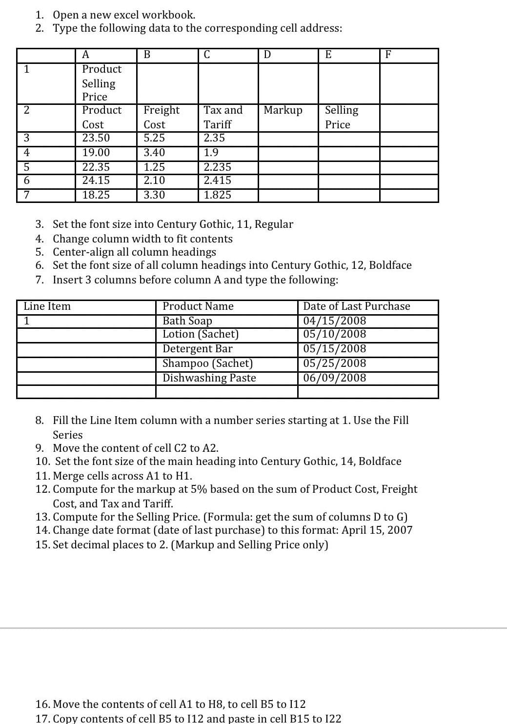
Transcribed Image Text:1. Open a new excel workbook.
2. Type the following data to the corresponding cell address:
A
В
E
F
1
Product
Selling
Price
2
Product
Freight
Тах and
Markup
Selling
Cost
Cost
Tariff
Price
23.50
5.25
2.35
4
19.00
3.40
1.9
2.235
2.415
1.25
22.35
24.15
2.10
7
18.25
3.30
1.825
3. Set the font size into Century Gothic, 11, Regular
4. Change column width to fit contents
5. Center-align all column headings
6. Set the font size of all column headings into Century Gothic, 12, Boldface
7. Insert 3 columns before column A and type the following:
Line Item
Product Name
Bath Soap
Lotion (Sachet)
Detergent Bar
Shampoo (Sachet)
Dishwashing Paste
Date of Last Purchase
04/15/2008
05/10/2008
05/15/2008
05/25/2008
06/09/2008
1
8. Fill the Line Item column with a number series starting at 1. Use the Fill
Series
9. Move the content of cell C2 to A2.
10. Set the font size of the main heading into Century Gothic, 14, Boldface
11. Merge cells across A1 to H1.
12. Compute for the markup at 5% based on the sum of Product Cost, Freight
Cost, and Tax and Tariff.
13. Compute for the Selling Price. (Formula: get the sum of columns D to G)
14. Change date format (date of last purchase) to this format: April 15, 2007
15. Set decimal places to 2. (Markup and Selling Price only)
16. Move the contents of cell A1 to H8, to cell B5 to I12
17. Copy contents of cell B5 to I12 and paste in cell B15 to 122
Expert Solution
This question has been solved!
Explore an expertly crafted, step-by-step solution for a thorough understanding of key concepts.

This is a popular solution!

Trending now
This is a popular solution!

Step by step
Solved in 2 steps with 3 images

Knowledge Booster


Learn more about
Need a deep-dive on the concept behind this application? Look no further. Learn more about this topic, accounting and related others by exploring similar questions and additional content below.Recommended textbooks for you
Excel Applications for Accounting Principles
Accounting
ISBN:
9781111581565
Author:
Gaylord N. Smith
Publisher:
Cengage Learning

Excel Applications for Accounting Principles
Accounting
ISBN:
9781111581565
Author:
Gaylord N. Smith
Publisher:
Cengage Learning