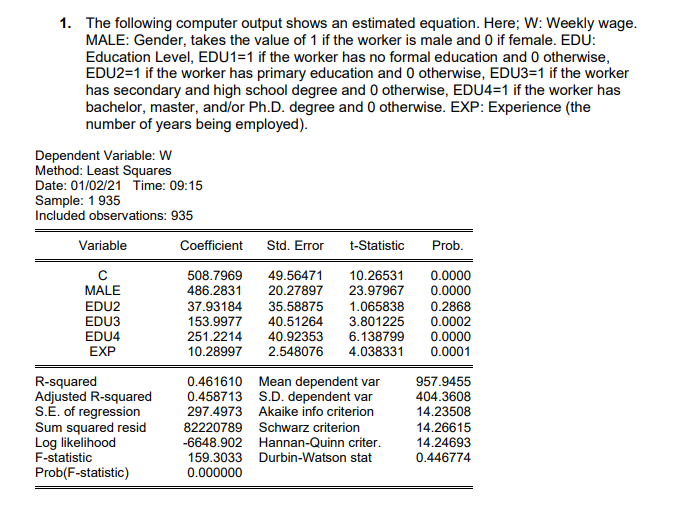
1. The following computer output shows an estimated equation. Here; W: Weekly wage. MALE: Gender, takes the value of 1 if the worker is male and 0 if female. EDU: Education Level, EDU1=1 if the worker has no formal education and 0 otherwise, EDU2=1 if the worker has primary education and 0 otherwise, EDU3=1 if the worker has secondary and high school degree and 0 otherwise, EDU4=1 if the worker has bachelor, master, and/or Ph.D. degree and 0 otherwise. EXP: Experience (the number of years being employed). Dependent Variable: W Method: Least Squares Date: 01/02/21 Time: 09:15 Sample: 1 935 Included observations: 935 Variable Coefficient Std. Error t-Statistic Prob. 508.7969 486.2831 37.93184 49.56471 10.26531 23.97967 0.0000 0.0000 MALE 20.27897 EDU2 EDU3 EDU4 EXP 153.9977 251.2214 10.28997 35.58875 40.51264 40.92353 2.548076 1.065838 3.801225 6.138799 4.038331 0.2868 0.0002 0.0000 0.0001 R-squared Adjusted R-squared S.É. of regression Sum squared resid Log likelihood F-statistic Prob(F-statistic) 0.461610 Mean dependent var 0.458713 S.D. dependent var 297.4973 Akaike info criterion 82220789 Schwarz criterion -6648.902 Hannan-Quinn criter. 159.3033 Durbin-Watson stat 0.000000 957.9455 404.3608 14.23508 14.26615 14.24693 0.446774
1. The following computer output shows an estimated equation. Here; W: Weekly wage. MALE: Gender, takes the value of 1 if the worker is male and 0 if female. EDU: Education Level, EDU1=1 if the worker has no formal education and 0 otherwise, EDU2=1 if the worker has primary education and 0 otherwise, EDU3=1 if the worker has secondary and high school degree and 0 otherwise, EDU4=1 if the worker has bachelor, master, and/or Ph.D. degree and 0 otherwise. EXP: Experience (the number of years being employed). Dependent Variable: W Method: Least Squares Date: 01/02/21 Time: 09:15 Sample: 1 935 Included observations: 935 Variable Coefficient Std. Error t-Statistic Prob. 508.7969 486.2831 37.93184 49.56471 10.26531 23.97967 0.0000 0.0000 MALE 20.27897 EDU2 EDU3 EDU4 EXP 153.9977 251.2214 10.28997 35.58875 40.51264 40.92353 2.548076 1.065838 3.801225 6.138799 4.038331 0.2868 0.0002 0.0000 0.0001 R-squared Adjusted R-squared S.É. of regression Sum squared resid Log likelihood F-statistic Prob(F-statistic) 0.461610 Mean dependent var 0.458713 S.D. dependent var 297.4973 Akaike info criterion 82220789 Schwarz criterion -6648.902 Hannan-Quinn criter. 159.3033 Durbin-Watson stat 0.000000 957.9455 404.3608 14.23508 14.26615 14.24693 0.446774

Linear Algebra: A Modern Introduction
4th Edition
ISBN:9781285463247
Author:David Poole
Publisher:David Poole
Chapter2: Systems Of Linear Equations
Section2.4: Applications
Problem 15EQ

Related questions
Question
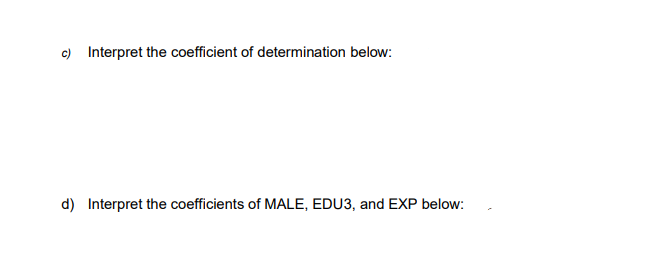
Transcribed Image Text:c) Interpret the coefficient of determination below:
d) Interpret the coefficients of MALE, EDU3, and EXP below:
Transcribed Image Text:1. The following computer output shows an estimated equation. Here; W: Weekly wage.
MALE: Gender, takes the value of 1 if the worker is male and 0 if female. EDU:
Education Level, EDU1=1 if the worker has no formal education and 0 otherwise,
EDU2=1 if the worker has primary education and 0 otherwise, EDU3=1 if the worker
has secondary and high school degree and 0 otherwise, EDU4=1 if the worker has
bachelor, master, and/or Ph.D. degree and 0 otherwise. EXP: Experience (the
number of years being employed).
Dependent Variable: W
Method: Least Squares
Date: 01/02/21 Time: 09:15
Sample: 1 935
Included observations: 935
Variable
Coefficient
Std. Error
t-Statistic
Prob.
508.7969
486.2831
49.56471
20.27897
10.26531
23.97967
0.0000
0.0000
0.2868
0.0002
0.0000
0.0001
MALE
EDU2
EDU3
EDU4
EXP
37.93184
153.9977
251.2214
10.28997
35.58875
40.51264
40.92353
2.548076
1.065838
3.801225
6.138799
4.038331
0.461610 Mean dependent var
0.458713 S.D. dependent var
297.4973 Akaike info criterion
957.9455
404.3608
14.23508
R-squared
Adjusted R-squared
S.É. of regression
Sum squared resid
Log likelihood
F-statistic
82220789 Schwarz criterion
-6648.902 Hannan-Quinn criter.
159.3033
0.000000
14.26615
14.24693
0.446774
Durbin-Watson stat
Prob(F-statistic)
Expert Solution
This question has been solved!
Explore an expertly crafted, step-by-step solution for a thorough understanding of key concepts.

This is a popular solution!

Trending now
This is a popular solution!

Step by step
Solved in 2 steps

Knowledge Booster


Learn more about
Need a deep-dive on the concept behind this application? Look no further. Learn more about this topic, statistics and related others by exploring similar questions and additional content below.Recommended textbooks for you
Linear Algebra: A Modern Introduction
Algebra
ISBN:
9781285463247
Author:
David Poole
Publisher:
Cengage Learning

Algebra & Trigonometry with Analytic Geometry
Algebra
ISBN:
9781133382119
Author:
Swokowski
Publisher:
Cengage
Linear Algebra: A Modern Introduction
Algebra
ISBN:
9781285463247
Author:
David Poole
Publisher:
Cengage Learning
Algebra & Trigonometry with Analytic Geometry
Algebra
ISBN:
9781133382119
Author:
Swokowski
Publisher:
Cengage