A manufacturer of chocolate candies uses machines to package candies as they move along a filling line. Although the packages are labeled as 8 ounces, the company wants the packages to contain a mean of 8.17 ounces so that virtually none of the packages contain less than 8 ounces. A sample of 50 packages is selected periodically, and the packaging process is stopped if there is evidence that the mean amount packaged is different from 8.17 ounces. Suppose that in a particular sample of 50 packages, the mean amount dispensed is 8.155 ounces, with a sample standard deviation of 0.056 ounce. Complete parts (a) and (b). Click here to view page 1 of the critical values for the t Distribution. Click here to view page 2 of the critical values for the t Distribution a. Is there evidence that the population mean amount is different from 8.17 ounces? (Use a 0.01 level of significance.) State the null and alternative hypotheses. Ho: HY H₁: HY (Type integers or decimals.) Identify the critical value(s). The critical value(s) is (are). (Round to four decimal places as needed. Use a comma to separate answers as needed.) Determine the test statistic. The test statistic is (Round to four decimal places as needed.) State the conclusion. Ho. There is evidence to conclude the population mean amount is different from 8.17 ounces
A manufacturer of chocolate candies uses machines to package candies as they move along a filling line. Although the packages are labeled as 8 ounces, the company wants the packages to contain a mean of 8.17 ounces so that virtually none of the packages contain less than 8 ounces. A sample of 50 packages is selected periodically, and the packaging process is stopped if there is evidence that the mean amount packaged is different from 8.17 ounces. Suppose that in a particular sample of 50 packages, the mean amount dispensed is 8.155 ounces, with a sample standard deviation of 0.056 ounce. Complete parts (a) and (b). Click here to view page 1 of the critical values for the t Distribution. Click here to view page 2 of the critical values for the t Distribution a. Is there evidence that the population mean amount is different from 8.17 ounces? (Use a 0.01 level of significance.) State the null and alternative hypotheses. Ho: HY H₁: HY (Type integers or decimals.) Identify the critical value(s). The critical value(s) is (are). (Round to four decimal places as needed. Use a comma to separate answers as needed.) Determine the test statistic. The test statistic is (Round to four decimal places as needed.) State the conclusion. Ho. There is evidence to conclude the population mean amount is different from 8.17 ounces

Glencoe Algebra 1, Student Edition, 9780079039897, 0079039898, 2018
18th Edition
ISBN:9780079039897
Author:Carter
Publisher:Carter
Chapter10: Statistics
Section10.3: Measures Of Spread
Problem 1GP

Related questions
Question
Critical Values of t. For a particular number of degrees of freedom, entry represents the critical value of t corresponding to the cumulative probability 1 minus alpha and a specified upper-tail area alpha.
Cumulative Probabilities
0.75 0.90 0.95 0.975 0.99 0.995
Upper-Tail Areas
Degrees of Freedom 0.25 0.10 0.05 0.025 0.01 0.005
1 1.0000 3.0777 6.3138 12.7062 31.8207 63.6574
2 0.8165 1.8856 2.9200 4.3027 6.9646 9.9248
3 0.7649 1.6377 2.3534 3.1824 4.5407 5.8409
4 0.7407 1.5332 2.1318 2.7764 3.7469 4.6041
5 0.7267 1.4759 2.0150 2.5706 3.3649 4.0322
6 0.7176 1.4398 1.9432 2.4469 3.1427 3.7074
7 0.7111 1.4149 1.8946 2.3646 2.9980 3.4995
8 0.7064 1.3968 1.8595 2.3060 2.8965 3.3554
9 0.7027 1.3830 1.8331 2.2622 2.8214 3.2498
10 0.6998 1.3722 1.8125 2.2281 2.7638 3.1693
11 0.6974 1.3634 1.7959 2.2010 2.7181 3.1058
12 0.6955 1.3562 1.7823 2.1788 2.6810 3.0545
13 0.6938 1.3502 1.7709 2.1604 2.6503 3.0123
14 0.6924 1.3450 1.7613 2.1448 2.6245 2.9768
15 0.6912 1.3406 1.7531 2.1315 2.6025 2.9467
16 0.6901 1.3368 1.7459 2.1199 2.5835 2.9208
17 0.6892 1.3334 1.7396 2.1098 2.5669 2.8982
18 0.6884 1.3304 1.7341 2.1009 2.5524 2.8784
19 0.6876 1.3277 1.7291 2.0930 2.5395 2.8609
20 0.6870 1.3253 1.7247 2.0860 2.5280 2.8453
21 0.6864 1.3232 1.7207 2.0796 2.5177 2.8314
22 0.6858 1.3212 1.7171 2.0739 2.5083 2.8188
23 0.6853 1.3195 1.7139 2.0687 2.4999 2.8073
24 0.6848 1.3178 1.7109 2.0639 2.4922 2.7969
25 0.6844 1.3163 1.7081 2.0595 2.4851 2.7874
26 0.6840 1.3150 1.7056 2.0555 2.4786 2.7787
27 0.6837 1.3137 1.7033 2.0518 2.4727 2.7707
28 0.6834 1.3125 1.7011 2.0484 2.4671 2.7633
29 0.6830 1.3114 1.6991 2.0452 2.4620 2.7564
30 0.6828 1.3104 1.6973 2.0423 2.4573 2.7500
31 0.6825 1.3095 1.6955 2.0395 2.4528 2.7440
32 0.6822 1.3086 1.6939 2.0369 2.4487 2.7385
33 0.6820 1.3077 1.6924 2.0345 2.4448 2.7333
34 0.6818 1.3070 1.6909 2.0322 2.4411 2.7284
35 0.6816 1.3062 1.6896 2.0301 2.4377 2.7238
36 0.6814 1.3055 1.6883 2.0281 2.4345 2.7195
37 0.6812 1.3049 1.6871 2.0262 2.4314 2.7154
38 0.6810 1.3042 1.6860 2.0244 2.4286 2.7116
39 0.6808 1.3036 1.6849 2.0227 2.4258 2.7079
40 0.6807 1.3031 1.6839 2.0211 2.4233 2.7045
41 0.6805 1.3025 1.6829 2.0195 2.4208 2.7012
42 0.6804 1.3020 1.6820 2.0181 2.4185 2.6981
43 0.6802 1.3016 1.6811 2.0167 2.4163 2.6951
44 0.6801 1.3011 1.6802 2.0154 2.4141 2.6923
45 0.6800 1.3006 1.6794 2.0141 2.4121 2.6896
46 0.6799 1.3002 1.6787 2.0129 2.4102 2.6870
47 0.6797 1.2998 1.6779 2.0117 2.4083 2.6846
48 0.6796 1.2994 1.6772 2.0106 2.4066 2.6822
Critical Values of t.
Cumulative Probabilities
0.75 0.90 0.95 0.975 0.99 0.995
Upper-Tail Areas
Degrees of Freedom 0.25 0.10 0.05 0.025 0.01 0.005
49 0.6795 1.2991 1.6766 2.0096 2.4049 2.6800
50 0.6794 1.2987 1.6759 2.0086 2.4033 2.6778
51 0.6793 1.2984 1.6753 2.0076 2.4017 2.6757
52 0.6792 1.2980 1.6747 2.0066 2.4002 2.6737
53 0.6791 1.2977 1.6741 2.0057 2.3988 2.6718
54 0.6791 1.2974 1.6736 2.0049 2.3974 2.6700
55 0.6790 1.2971 1.6730 2.0040 2.3961 2.6682
56 0.6789 1.2969 1.6725 2.0032 2.3948 2.6665
57 0.6788 1.2966 1.6720 2.0025 2.3936 2.6649
58 0.6787 1.2963 1.6716 2.0017 2.3924 2.6633
59 0.6787 1.2961 1.6711 2.0010 2.3912 2.6618
60 0.6786 1.2958 1.6706 2.0003 2.3901 2.6603
61 0.6785 1.2956 1.6702 1.9996 2.3890 2.6589
62 0.6785 1.2954 1.6698 1.9990 2.3880 2.6575
63 0.6784 1.2951 1.6694 1.9983 2.3870 2.6561
64 0.6783 1.2949 1.6690 1.9977 2.3860 2.6549
65 0.6783 1.2947 1.6686 1.9971 2.3851 2.6536
66 0.6782 1.2945 1.6683 1.9966 2.3842 2.6524
67 0.6782 1.2943 1.6679 1.9960 2.3833 2.6512
68 0.6781 1.2941 1.6676 1.9955 2.3824 2.6501
69 0.6781 1.2939 1.6672 1.9949 2.3816 2.6490
70 0.6780 1.2938 1.6669 1.9944 2.3808 2.6479
71 0.6780 1.2936 1.6666 1.9939 2.3800 2.6469
72 0.6779 1.2934 1.6663 1.9935 2.3793 2.6459
73 0.6779 1.2933 1.6660 1.9930 2.3785 2.6449
74 0.6778 1.2931 1.6657 1.9925 2.3778 2.6439
75 0.6778 1.2929 1.6654 1.9921 2.3771 2.6430
76 0.6777 1.2928 1.6652 1.9917 2.3764 2.6421
77 0.6777 1.2926 1.6649 1.9913 2.3758 2.6412
78 0.6776 1.2925 1.6646 1.9908 2.3751 2.6403
79 0.6776 1.2924 1.6644 1.9905 2.3745 2.6395
80 0.6776 1.2922 1.6641 1.9901 2.3739 2.6387
81 0.6775 1.2921 1.6639 1.9897 2.3733 2.6379
82 0.6775 1.2920 1.6636 1.9893 2.3727 2.6371
83 0.6775 1.2918 1.6634 1.9890 2.3721 2.6364
84 0.6774 1.2917 1.6632 1.9886 2.3716 2.6356
85 0.6774 1.2916 1.6630 1.9883 2.3710 2.6349
86 0.6774 1.2915 1.6628 1.9879 2.3705 2.6342
87 0.6773 1.2914 1.6626 1.9876 2.3700 2.6335
88 0.6773 1.2912 1.6624 1.9873 2.3695 2.6329
89 0.6773 1.2911 1.6622 1.9870 2.3690 2.6322
90 0.6772 1.2910 1.6620 1.9867 2.3685 2.6316
91 0.6772 1.2909 1.6618 1.9864 2.3680 2.6309
92 0.6772 1.2908 1.6616 1.9861 2.3676 2.6303
93 0.6771 1.2907 1.6614 1.9858 2.3671 2.6297
94 0.6771 1.2906 1.6612 1.9855 2.3667 2.6291
95 0.6771 1.2905 1.6611 1.9853 2.3662 2.6286
96 0.6771 1.2904 1.6609 1.9850 2.3658 2.6280
97 0.6770 1.2903 1.6607 1.9847 2.3654 2.6275
98 0.6770 1.2902 1.6606 1.9845 2.3650 2.6269
99 0.6770 1.2902 1.6604 1.9842 2.3646 2.6264
100 0.6770 1.2901 1.6602 1.9840 2.3642 2.6259
110 0.6767 1.2893 1.6588 1.9818 2.3607 2.6213
120 0.6765 1.2886 1.6577 1.9799 2.3578 2.6174
infinity 0.6745 1.2816 1.6449 1.9600 2.3263 2.5758
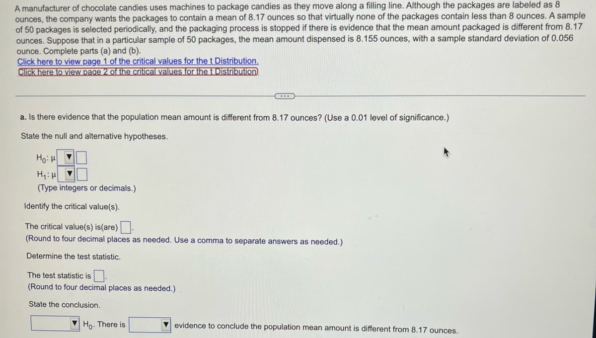
Transcribed Image Text:A manufacturer of chocolate candies uses machines to package candies as they move along a filling line. Although the packages are labeled as 8
ounces, the company wants the packages to contain a mean of 8.17 ounces so that virtually none of the packages contain less than 8 ounces. A sample
of 50 packages is selected periodically, and the packaging process is stopped if there is evidence that the mean amount packaged is different from 8.17
ounces. Suppose that in a particular sample of 50 packages, the mean amount dispensed is 8.155 ounces, with a sample standard deviation of 0.056
ounce. Complete parts (a) and (b).
Click here to view page 1 of the critical values for the t Distribution.
Click here to view page 2 of the critical values for the t Distribution
a. Is there evidence that the population mean amount is different from 8.17 ounces? (Use a 0.01 level of significance.)
State the null and alternative hypotheses.
Hoi H
H₁: H
▼
(Type integers or decimals.)
...
Identify the critical value(s).
The critical value(s) is (are).
(Round to four decimal places as needed. Use a comma to separate answers as needed.)
Determine the test statistic.
The test statistic is
(Round to four decimal places as needed.)
State the conclusion.
Ho. There is
evidence to conclude the population mean amount is different from 8.17 ounces.
Transcribed Image Text:A manufacturer of chocolate candies uses machines to package candies as they move along a filling line. Although the packages are labeled as 8
ounces, the company wants the packages to contain a mean of 8.17 ounces so that virtually none of the packages contain less than 8 ounces. A sample
of 50 packages is selected periodically, and the packaging process is stopped if there is evidence that the mean amount packaged is different from 8.17
ounces. Suppose that in a particular sample of 50 packages, the mean amount dispensed is 8.155 ounces, with a sample standard deviation of 0.056
ounce. Complete parts (a) and (b).
Click here to view page 1 of the critical values for the t Distribution.
Click here to view page 2 of the critical values for the t Distribution
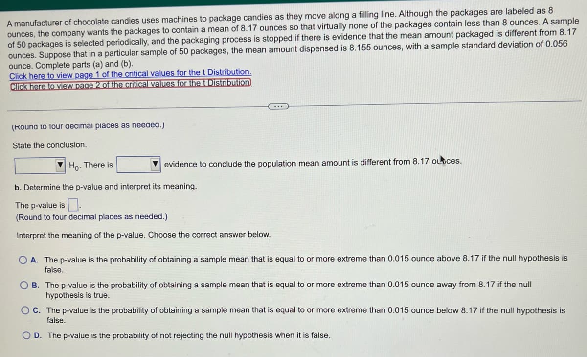
(Kouna to Tour decimal places as needea.)
State the conclusion.
evidence to conclude the population mean amount is different from 8.17 outices.
Ho. There is
b. Determine the p-value and interpret its meaning.
The p-value is.
(Round to four decimal places as needed.)
Interpret the meaning of the p-value. Choose the correct answer below.
OA. The p-value is the probability of obtaining a sample mean that is equal to or more extreme than 0.015 ounce above 8.17 if the null hypothesis is
false.
OB. The p-value is the probability of obtaining a sample mean that is equal to or more extreme than 0.015 ounce away from 8.17 if the null
hypothesis is true.
OC. The p-value is the probability of obtaining a sample mean that is equal to or more extreme than 0.015 ounce below 8.17 if the null hypothesis is
false.
D. The p-value is the probability of not rejecting the null hypothesis when it is false.
Expert Solution
This question has been solved!
Explore an expertly crafted, step-by-step solution for a thorough understanding of key concepts.

This is a popular solution!

Trending now
This is a popular solution!

Step by step
Solved in 3 steps with 3 images

Recommended textbooks for you
Glencoe Algebra 1, Student Edition, 9780079039897…
Algebra
ISBN:
9780079039897
Author:
Carter
Publisher:
McGraw Hill
Glencoe Algebra 1, Student Edition, 9780079039897…
Algebra
ISBN:
9780079039897
Author:
Carter
Publisher:
McGraw Hill