Determine the probability of each of the following by using the standard normal distribution table. (b) P(Z<-1.21) P(Z<0.76)
Determine the probability of each of the following by using the standard normal distribution table. (b) P(Z<-1.21) P(Z<0.76)

College Algebra
7th Edition
ISBN:9781305115545
Author:James Stewart, Lothar Redlin, Saleem Watson
Publisher:James Stewart, Lothar Redlin, Saleem Watson
Chapter9: Counting And Probability
Section9.3: Binomial Probability
Problem 2E: If a binomial experiment has probability p success, then the probability of failure is...

Related questions
Question
Determine the probability of each of the following by using the standard normal distribution table
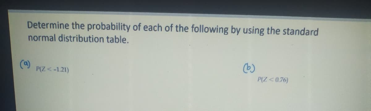
Transcribed Image Text:Determine the probability of each of the following by using the standard
normal distribution table.
()
P(Z<-1.21)
(b)
P(Z<0.76)
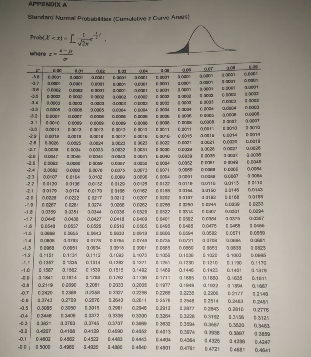
Transcribed Image Text:APPENDIXA
Standard Normal Probabilities (Cumulative z Curve Areas)
Prob(X <x) =
where z=
0.06
0.07
0.08
0.09
z*
0.00
0.01
0.02
0.03
0.04
0.05
0.0001
0.0001
0.0001
-3.8
0.0001
0.0001
0.0001
0.0001
0.0001
0.0001
0.0001
0.0001
0.0001
0.0001
-3.7
0.0001
0.0001
0.0001
0.0001
0.0001
0.0001
0.0001
0.0001
0.0001
-3.6
0.0002
0.0002
0.0001
0.0001
0.0001
0.0001
0.0001
0.0001
0.0002
0.0002
-3.5
0.0002
0.0002
0.0002
0.0002
0.0002
0.0002
0.0002
0.0002
3.4
0.0003
0.0003
0.0003
0.0003
0.0003
0.0002
0.0003
0.0003
0.0003
0.0003
-3.3
0.0005
0.0004
0.0004
0.0004
0.0003
0.0005
0.0005
0.0004
0.0004
0.0004
-3.2
0.0005
0.0005
0.0005
0.0006
0.0009
0.0007
0.0007
0.0006
0.0006
0.0006
0.0006
-3.1
0.0010
0.0009
0.0009
0.0008
0.0008
0.0008
0.0008
0.0007
0.0007
-3.0
0.0013
0.0013
0.0013
0.0012
0.0012
0.0011
0.0011
0.0011
0.0010
0.0010
-2.9
0.0019
0.0018
0.0018
0.0017
0.0016
0.0016
0.0015
0.0015
0.0014
0.0014
-2.8
0.0026
0.0025
0.0024
0.0023
0.0023
0.0022
0.0021
0.0021
0.0020
0.0019
-2.7
0.0035
0.0034
0.0033
0.0032
0.0031
0.0030
0.0029
0.0028
0.0027
0.0026
-2.6
0.0047
0.0043
0.0040
0.0039
0.0038
0.0037
0.0036
0.0045
0.0044
0.0041
-2.5
0.0062
0.0060
0.0059
0.0057
0.0055
0.0054
0.0052
0.0051
0.0049
0.0048
-2.4
0.0082
0.0080
0.0078
0.0075
0.0073
0.0071
0.0069
0.0068
0.0066
0.0064
-2.3
0.0107
0.0104
0.0102
0.0099
0.0096
0.0094
0.0091
0.0089
0.0087
0.0084
-2.2
0.0139
0.0136
0.0132
0.0129
0.0125
0.0122
0.0119
0.0116
0.0113
0.0110
-2.1
0.0179
0.0174
0.0170
0.0166
0.0162
0.0158
0.0154
0.0150
0.0146
0.0143
-2.0
0.0228
0.0222
0.0217
0.0212
0.0207
0.0202
0.0197
0.0192
0.0188
0.0183
-1.9
0.0287
0.0281
0.0274
0.0268
0.0262
0.0256
0.0250
0.0244
0.0239
0.0233
-1.8
0.0359
0.0351
0.0344
0.0336
0.0329
0.0322
0.0314
0.0307
0.0301
0.0294
-1.7
0.0446
0.0436
0.0427
0.0418
0.0409
0.0401
0.0392
0.0384
0.0375
0.0367
-1.6
0.0548
0.0537
0.0526
0.0516
0.0505
0.0495
0.0485
0.0475
0.0465
0.0455
-1.5
0.0668
0.0655
0.0643
0.0630
0.0618
0.0606
0.0594
0.0582
0.0571
0.0559
-1.4
0.0808
0.0793
0.0778
0.0764
0.0749
0.0735
0.0721
0.0708
0.0694
0.0681
-1.3
0.0968
0.0951
0.0934
0.0918
0.0901
0.0885
0.0869
0.0853
0.0838
0.0823
-1.2
0.1151
0.1131
0.1112
0.1093
0.1075
0.1056
0.1038
0.1020
0.1003
0.0985
-1.1
0.1357
0.1335
0.1314
0.1292
0.1271
0.1251
0.1230
0.1210
0.1190
0.1170
-1.0
0.1587
0.1562
0.1539
0.1515
0.1492
0.1469
0.1446
0.1423
0.1401
0.1379
-0.9
0.1841
0.1814
0.1788
0.1762
0.1736
0.1711
0.1685
0.1660
0.1635
0.1611
-0.8
0.2119
0.2090
0.2061
0.2033
0.2005
0.1977
0.1949
0.1922
0.1894
0.1867
-0.7
0.2420
0.2389
0.2358
0.2327
0.2296
0.2266
0.2236
0.2206
0.2177
0.2148
-0.6
0.2743
0.2709
0.2676
0.2643
0.2611
0.2578
0.2546
0.2514
0.2483
0.2451
-0.5
0.3085
0.3050
0.3015
0.2981
0.2946
0.2912
0.2877
0.2843
0.2810
0.2776
-0.4
0.3446
0.3409
0.3372
0.3336
0.3300
0.3264
0.3228
0.3192
0.3156
0.3121
0.3
0.3821
0.3783
0.3745
0.3707
0.3669
0.3632
0.3594
0.3557
0.3520
0.3483
-0.2
0.4207
0.4168
0.4129
0.4090
0.4052
0.4013
0.3974
0.3936
0.3897
0.3859
-0.1
0.4602
0.4562
0.4522
0.4483
0.4443
0.4404
0.4364
0.4325
0.4286
0.4247
-0.0
0.5000
0.4960
0.4920
0.4880
0.4840
0.4801
0.4761
0.4721
0.4681
0.4641
Expert Solution
This question has been solved!
Explore an expertly crafted, step-by-step solution for a thorough understanding of key concepts.

Step by step
Solved in 2 steps with 2 images

Recommended textbooks for you
College Algebra
Algebra
ISBN:
9781305115545
Author:
James Stewart, Lothar Redlin, Saleem Watson
Publisher:
Cengage Learning

College Algebra
Algebra
ISBN:
9781305115545
Author:
James Stewart, Lothar Redlin, Saleem Watson
Publisher:
Cengage Learning