Digital Controls, Inc. (DCI), manufactures tvo models of a radar gun used by police to monitor the speed of automobiles. Model A has an accuracy of plus or minus 1 mile per hour, vhereas the smaller model 8 has an accuracy of plus or minus 3 miles per hour. For the next week, the company has orders for 100 units of model A and 150 units of model B. Although DCI purchases all the electronic components used in both models, the plastic cases for both models are manufactured at a DCI plant in Nevark, New Jersey. Each model A case requires 4 minutes of injection-molding time and 6 minutes of assembly time. Each model B case requires 3 minutes of injection-molding time and 8 minutes of assembly time. For next week, the Newark plant has 600 minutes of injection-molding time available and 1.080 minutes of assembly time available. The manufacturing cost is $10 per case for model A and $6 per case for model B. Depending upon demand and the time available at the Newark plant, DCI occasionally purchases cases for one or both models from an outside supplier in order to fill customer orders that could not be filled othervise. The purchase cost is $14 for each model A case and $9 for each model B case. Management vants to develop a minimum cost plan that vill determine how many cases of each model should be produced at the Newark plant and how many cases of each model should be purchased. The folloving decision variables were used to formulate a linear programming model for this problem: AM = number of cases of model A manufactured BM = number of cases of model B manufactured AP = number of cases of model A purchased BP = number of cases of model B purchased The linear programming model that can be used to solve this problem is as follows: Min 10AM + 6BM + 14AP + 9BP s.t. 1AM + 1AP + = 100 Demand for model A 1BM + 18P - 150 Demand for model B s 600 s 1,080 Injection molding time Assembly time 4AM + 3BM 6AM + 8BM AM, BM, AP, BP 20 Refer to the computer solution below. Optimal Objective Value = 2170.00000 Variable Value Reduced Coss AM 100.00000 0.00000 BM 60.00000 0.00000 AP 0.00000 1.75000 BP 90.00000 0.00000 Constraint 9lack/Surplus Dual Value 0.00000 -12.25000 0.00000 -9.00000 20.00000 0.00000 0.00000 0.37500 Allowable Allowable Objecsáve Coefficiens Variable Increase Decrease AM 10.00000 1.75000 Infinite BM 6.00000 3.00000 2.33333 AP 14.00000 Infinise 1.75000 9.00000 2.33333 3.00000 RH3 Allowable Allowable Constraint Value Increase Deczease 100.00000 11.42057 100.00000 150.00000 Infinite 90.00000 600.00000 Infinite 20.00000 1,080.00000 53.33333 480.00000 (a) Interpret the ranges of optimality for the objective function coefficients. O f multiple changes are made to the injection molding time or assembly time for either model case vithin their respective allowable ranges, the optimal solution vill not change. O If a single change to the manufacturing cost or purchase cost for either model case is within the allowable range, the optimal solution vill not change. If multiple changes are made to the manufacturing or purchase costs for either model case vithin their respective allowable ranges, the optimal solution vill not change. O If a single change to the injection molding time or assembly time for either model case is vithin the allovable range, the optimal solution vill not change. (b) Suppose that the manufacturing cost increases to $11.50 per case for model A. Would the optimal solution change? Yes, it is necessary to solve the model again. O No, the optimal solution remains the same. What is the new optimal solution? at (AM, BM, AP, BP) = (c) Suppose that the manufacturing cost increases to $11.50 per case for model A and the manufacturing cost for model B decreases to $4 per unit. Would the optimal solution change? O Yes, it is necessary to solve the model again. O No, the optimal solution remains the same. What is the new optimal solution? at (AM, BM, AP, BP) =
Digital Controls, Inc. (DCI), manufactures tvo models of a radar gun used by police to monitor the speed of automobiles. Model A has an accuracy of plus or minus 1 mile per hour, vhereas the smaller model 8 has an accuracy of plus or minus 3 miles per hour. For the next week, the company has orders for 100 units of model A and 150 units of model B. Although DCI purchases all the electronic components used in both models, the plastic cases for both models are manufactured at a DCI plant in Nevark, New Jersey. Each model A case requires 4 minutes of injection-molding time and 6 minutes of assembly time. Each model B case requires 3 minutes of injection-molding time and 8 minutes of assembly time. For next week, the Newark plant has 600 minutes of injection-molding time available and 1.080 minutes of assembly time available. The manufacturing cost is $10 per case for model A and $6 per case for model B. Depending upon demand and the time available at the Newark plant, DCI occasionally purchases cases for one or both models from an outside supplier in order to fill customer orders that could not be filled othervise. The purchase cost is $14 for each model A case and $9 for each model B case. Management vants to develop a minimum cost plan that vill determine how many cases of each model should be produced at the Newark plant and how many cases of each model should be purchased. The folloving decision variables were used to formulate a linear programming model for this problem: AM = number of cases of model A manufactured BM = number of cases of model B manufactured AP = number of cases of model A purchased BP = number of cases of model B purchased The linear programming model that can be used to solve this problem is as follows: Min 10AM + 6BM + 14AP + 9BP s.t. 1AM + 1AP + = 100 Demand for model A 1BM + 18P - 150 Demand for model B s 600 s 1,080 Injection molding time Assembly time 4AM + 3BM 6AM + 8BM AM, BM, AP, BP 20 Refer to the computer solution below. Optimal Objective Value = 2170.00000 Variable Value Reduced Coss AM 100.00000 0.00000 BM 60.00000 0.00000 AP 0.00000 1.75000 BP 90.00000 0.00000 Constraint 9lack/Surplus Dual Value 0.00000 -12.25000 0.00000 -9.00000 20.00000 0.00000 0.00000 0.37500 Allowable Allowable Objecsáve Coefficiens Variable Increase Decrease AM 10.00000 1.75000 Infinite BM 6.00000 3.00000 2.33333 AP 14.00000 Infinise 1.75000 9.00000 2.33333 3.00000 RH3 Allowable Allowable Constraint Value Increase Deczease 100.00000 11.42057 100.00000 150.00000 Infinite 90.00000 600.00000 Infinite 20.00000 1,080.00000 53.33333 480.00000 (a) Interpret the ranges of optimality for the objective function coefficients. O f multiple changes are made to the injection molding time or assembly time for either model case vithin their respective allowable ranges, the optimal solution vill not change. O If a single change to the manufacturing cost or purchase cost for either model case is within the allowable range, the optimal solution vill not change. If multiple changes are made to the manufacturing or purchase costs for either model case vithin their respective allowable ranges, the optimal solution vill not change. O If a single change to the injection molding time or assembly time for either model case is vithin the allovable range, the optimal solution vill not change. (b) Suppose that the manufacturing cost increases to $11.50 per case for model A. Would the optimal solution change? Yes, it is necessary to solve the model again. O No, the optimal solution remains the same. What is the new optimal solution? at (AM, BM, AP, BP) = (c) Suppose that the manufacturing cost increases to $11.50 per case for model A and the manufacturing cost for model B decreases to $4 per unit. Would the optimal solution change? O Yes, it is necessary to solve the model again. O No, the optimal solution remains the same. What is the new optimal solution? at (AM, BM, AP, BP) =

Purchasing and Supply Chain Management
6th Edition
ISBN:9781285869681
Author:Robert M. Monczka, Robert B. Handfield, Larry C. Giunipero, James L. Patterson
Publisher:Robert M. Monczka, Robert B. Handfield, Larry C. Giunipero, James L. Patterson
ChapterC: Cases
Section: Chapter Questions
Problem 5.1SC: Scenario 3 Ben Gibson, the purchasing manager at Coastal Products, was reviewing purchasing...

Related questions
Question
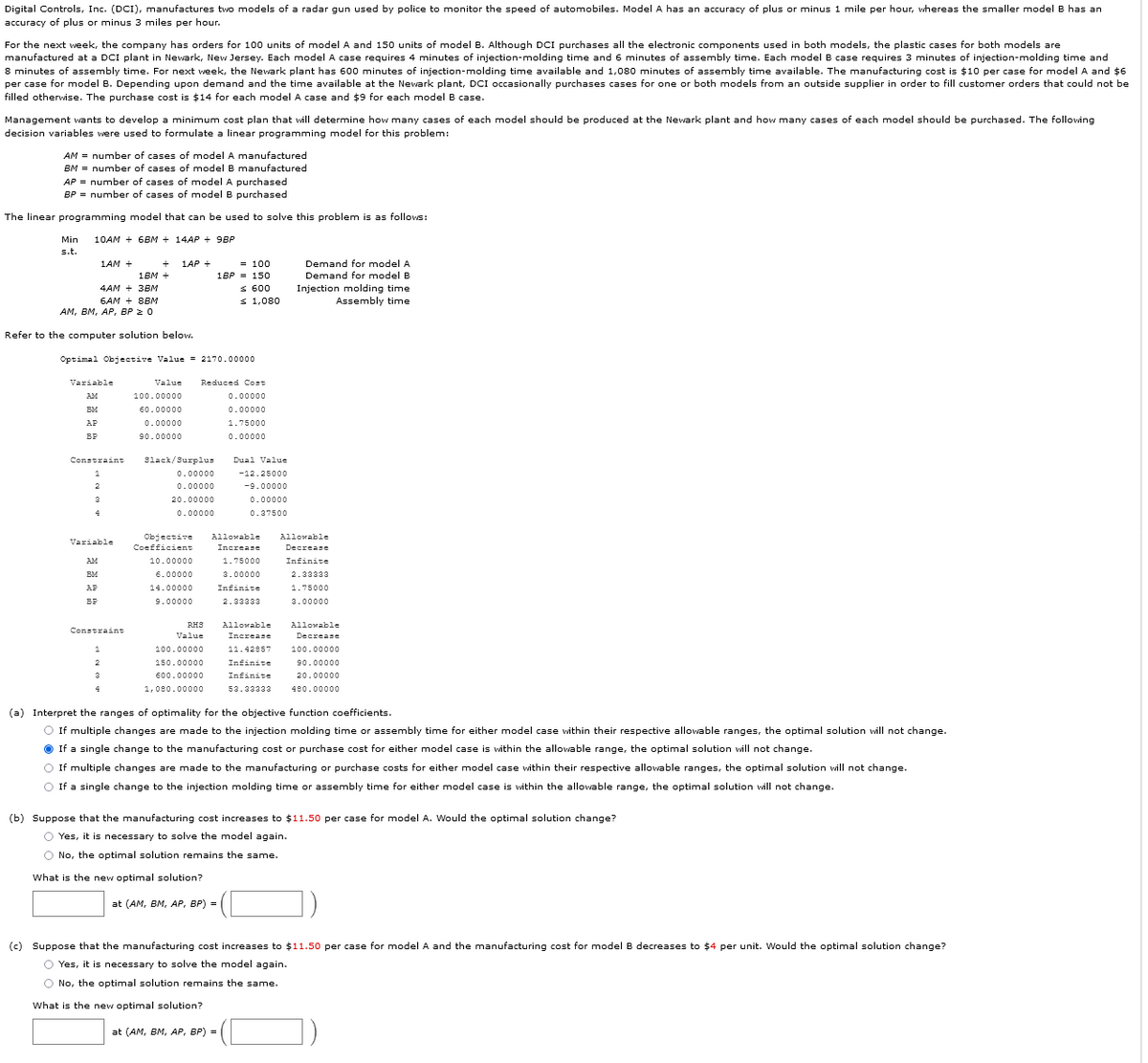
Transcribed Image Text:Digital Controls, Inc. (DCI), manufactures two models of a radar gun used by police to monitor the speed of automobiles. Model A has an accuracy of plus or minus 1 mile per hour, whereas the smaller model B has an
accuracy of plus or minus
miles per hour.
For the next week, the company has orders for 100 units of model A and 150 units of model B. Although DCI purchases all the electronic components used in both models, the plastic cases for both models are
manufactured at a DCI plant in Newark, New Jersey. Each model A case requires 4 minutes of injection-molding time and 6 minutes of assembly time. Each model B case requires 3 minutes of injection-molding time and
8 minutes of assembly time. For next week, the Newark plant has 600 minutes of injection-molding time available and 1,080 minutes of assembly time available. The manufacturing cost is $10 per case for model A and $6
per case for model B. Depending upon demand and the time available at the Newark plant, DCI occasionally purchases cases for one or both models from an outside supplier in order to fill customer orders that could not be
filled otherwise. The purchase cost is $14 for each model A case and $9 for each model B case.
Management wants to develop a minimum cost plan that will determine how many cases of each model should be produced at the Newark plant and how many cases of each model should be purchased. The following
decision variables were used to formulate a linear programming model for this problem:
AM = number of cases of model
manufactured
BM = number of cases of model B manufactured
AP = number of cases of model A purchased
BP = number of cases of model B purchased
The linear programming model that can be used to solve this problem is as follows:
Min
10AM + 6BM + 14AP + 9BP
s.t.
= 100
1BP = 150
1AM +
1AP +
Demand for model A
1BM +
Demand for model B
S 600
s 1,080
Injection molding time
Assembly time
4AM + 3BM
6AM + 8BM
АМ, Вм, АР, ВP 2 0
Refer to the computer solution below.
Optimal Objective Value = 2170.00000
Variable
Value
Reduced Cost
AM
100.00000
0.00000
EM
60.00000
0.00000
AP
0.00000
1.75000
90.00000
0.00000
Constraint
3lack/Surplus
Dual Value
0.00000
-12.25000
0.00000
-9.00000
20.00000
0.00000
0.00000
0.37500
Objective
Allowable
Allowable
Variable
Coefficient
Increase
Decrease
10.00000
1.75000
Infinite
EM
6.00000
3.00000
2.33333
AF
14.00000
Infinite
1.75000
BP
9.00000
2.33333
3.00000
RHS
Allowable
Allowable
Constraint
Value
Increase
Decrease
100.00000
11.42857
100.00000
150.00000
Infinite
90.00000
600.00000
Infinite
20.00000
1,080.00000
53.33333
480.00000
(a) Interpret the ranges of optimality for the objective function coefficients.
O If multiple changes are made to the injection molding time or assembly time for either model case within their respective allowable ranges, the optimal solution vill not change.
O If a single change to the manufacturing cost or purchase cost for either model case is within the allowable range, the optimal solution vill not change.
O If multiple changes are made to the manufacturing or purchase costs for either model case within their respective allowable ranges, the optimal solution will not change.
O If a single change to the injection molding time or assembly time for either model case is within the allowable range, the optimal solution vill not change.
(b) Suppose that the manufacturing cost increases to $i1.50 per case for model A. Would the optimal solution change?
O Yes, it is necessary to solve the model again.
O No, the optimal solution remains the same.
What is the new optimal solution?
at (AM, BM, AP, BP) =
(c) Suppose that the manufacturing cost increases to $11.50 per case for model A and the manufacturing cost for model B decreases to $4 per unit. Would the optimal solution change?
O Yes, it is necessary to solve the model again.
O No, the optimal solution remains the same.
What is the new optimal solution?
at (AM, BM, AP, BP) =
Expert Solution
This question has been solved!
Explore an expertly crafted, step-by-step solution for a thorough understanding of key concepts.

This is a popular solution!

Trending now
This is a popular solution!

Step by step
Solved in 2 steps with 3 images

Recommended textbooks for you
Purchasing and Supply Chain Management
Operations Management
ISBN:
9781285869681
Author:
Robert M. Monczka, Robert B. Handfield, Larry C. Giunipero, James L. Patterson
Publisher:
Cengage Learning

Practical Management Science
Operations Management
ISBN:
9781337406659
Author:
WINSTON, Wayne L.
Publisher:
Cengage,
Purchasing and Supply Chain Management
Operations Management
ISBN:
9781285869681
Author:
Robert M. Monczka, Robert B. Handfield, Larry C. Giunipero, James L. Patterson
Publisher:
Cengage Learning
Practical Management Science
Operations Management
ISBN:
9781337406659
Author:
WINSTON, Wayne L.
Publisher:
Cengage,