How did the slope (z) and y-intercept (b) values vary between the communities you sampled? Explain any similarities or differences. How did the Shannon-Wiener diversity indices for the largest nested plots (625 m2) differ between communities? This value typically ranges from 0.5–3, in which higher values reflect greater species richness and/or a more equitable distribution of species, whereas lower values reflect lower species richness and/or greater dominance by fewer species. Please provide your result and explain it in this context.
How did the slope (z) and y-intercept (b) values vary between the communities you sampled? Explain any similarities or differences. How did the Shannon-Wiener diversity indices for the largest nested plots (625 m2) differ between communities? This value typically ranges from 0.5–3, in which higher values reflect greater species richness and/or a more equitable distribution of species, whereas lower values reflect lower species richness and/or greater dominance by fewer species. Please provide your result and explain it in this context.
Applications and Investigations in Earth Science (9th Edition)
9th Edition
ISBN:9780134746241
Author:Edward J. Tarbuck, Frederick K. Lutgens, Dennis G. Tasa
Publisher:Edward J. Tarbuck, Frederick K. Lutgens, Dennis G. Tasa
Chapter1: The Study Of Minerals
Section: Chapter Questions
Problem 1LR

Related questions
Question
I need help with the following!
How did the slope (z) and y-intercept (b) values vary between the communities you sampled? Explain any similarities or differences.
How did the Shannon-Wiener diversity indices for the largest nested plots (625 m2) differ between communities? This value typically ranges from 0.5–3, in which higher values reflect greater species richness and/or a more equitable distribution of species, whereas lower values reflect lower species richness and/or greater dominance by fewer species. Please provide your result and explain it in this context.
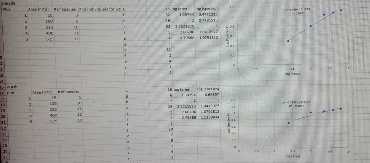
Transcribed Image Text:Bajada
1.2
Plot
Area (m^2)
# of species # of individuals for 625 c
15 log (area)
log (species)
y3D0.448x-0.1238
R =0.9682
25
3
32
1.39794
0.4771213
1
100
6.
16
0.7781513
3
225
10
53
2.3521825
0.8
4.
400
11
2.60206
1.0413927
0.6
625
12
2.79588
1.0791812
a
04
11
2
0.2
k
4
1
1
0.5
15
2.5
3
j
Log (Area)
14
15 Wash
16 log (area)
log (species)
16 Plot
Area (m^2)
# of species
1.39794
0.69897
17
25
7
1
1.4
100
10
¥=D0.2867x + 0.3474
18
28
2.3521825
1.0413927
R= 0.9051
1.2
19
3
225
11
3
2.60206
1.0791812
400
12
a
1
20
4.
2.79588
1.1139434
%23
625
13
0.B
21
0.6
22
28
0.4
23
7
24
8.
0.2
e
25
26
0.5
15
2.5
27
Log (Area)
28
Log (Species #)
Log(Species #)
0CO
2
2.
12
5.
2.
5.
Expert Solution
This question has been solved!
Explore an expertly crafted, step-by-step solution for a thorough understanding of key concepts.

Step by step
Solved in 2 steps

Recommended textbooks for you
Applications and Investigations in Earth Science …
Earth Science
ISBN:
9780134746241
Author:
Edward J. Tarbuck, Frederick K. Lutgens, Dennis G. Tasa
Publisher:
PEARSON

Exercises for Weather & Climate (9th Edition)
Earth Science
ISBN:
9780134041360
Author:
Greg Carbone
Publisher:
PEARSON
Environmental Science
Earth Science
ISBN:
9781260153125
Author:
William P Cunningham Prof., Mary Ann Cunningham Professor
Publisher:
McGraw-Hill Education
Applications and Investigations in Earth Science …
Earth Science
ISBN:
9780134746241
Author:
Edward J. Tarbuck, Frederick K. Lutgens, Dennis G. Tasa
Publisher:
PEARSON
Exercises for Weather & Climate (9th Edition)
Earth Science
ISBN:
9780134041360
Author:
Greg Carbone
Publisher:
PEARSON
Environmental Science
Earth Science
ISBN:
9781260153125
Author:
William P Cunningham Prof., Mary Ann Cunningham Professor
Publisher:
McGraw-Hill Education
Earth Science (15th Edition)
Earth Science
ISBN:
9780134543536
Author:
Edward J. Tarbuck, Frederick K. Lutgens, Dennis G. Tasa
Publisher:
PEARSON
Environmental Science (MindTap Course List)
Earth Science
ISBN:
9781337569613
Author:
G. Tyler Miller, Scott Spoolman
Publisher:
Cengage Learning
Physical Geology
Earth Science
ISBN:
9781259916823
Author:
Plummer, Charles C., CARLSON, Diane H., Hammersley, Lisa
Publisher:
Mcgraw-hill Education,