Q2B - Plotting 1 Plot the data from the previous question along with a trendline. Make sure to include proper labels on the axes, but you do not require a title or caption for this plot. In [183]: N import matplotlib.pyplot as plt import numpy as np plt.figure(figsize=(8,4)) import matplotlib.pyplot as plt import pandas as pd from scipy.optimize import curve_fit import numpy as np samplex = np.linspace(e, 5e, 26) + np.random.normal(scale = 0.2, size = 26) sampley = 3 * samplex + 4 + np.random.normal (scale = 4, size = 26) print(sampleY) def obj(x,p,q): return p*x + q ans2 = curve_fit(obj, samplex, sampleY) ans1 p,q = ans1 print('Value of slope : ',p) print('Value of intercept : ',9) print('Value of uncertainity : ',np.sqrt(np.mean(np.power(sampley-(p*samplex +q),2))))
Q2B - Plotting 1 Plot the data from the previous question along with a trendline. Make sure to include proper labels on the axes, but you do not require a title or caption for this plot. In [183]: N import matplotlib.pyplot as plt import numpy as np plt.figure(figsize=(8,4)) import matplotlib.pyplot as plt import pandas as pd from scipy.optimize import curve_fit import numpy as np samplex = np.linspace(e, 5e, 26) + np.random.normal(scale = 0.2, size = 26) sampley = 3 * samplex + 4 + np.random.normal (scale = 4, size = 26) print(sampleY) def obj(x,p,q): return p*x + q ans2 = curve_fit(obj, samplex, sampleY) ans1 p,q = ans1 print('Value of slope : ',p) print('Value of intercept : ',9) print('Value of uncertainity : ',np.sqrt(np.mean(np.power(sampley-(p*samplex +q),2))))

Computer Networking: A Top-Down Approach (7th Edition)
7th Edition
ISBN:9780133594140
Author:James Kurose, Keith Ross
Publisher:James Kurose, Keith Ross
Chapter1: Computer Networks And The Internet
Section: Chapter Questions
Problem R1RQ: What is the difference between a host and an end system? List several different types of end...

Related questions
Question
100%
Plz use the given code to plot the fit plz
![Markdown
O nbdiff l
123.771659
128.10434637 140.17173392 146.29001843 152.50565637
152.95840512]
Value of slope :
Value of intercept :
Value of uncertainity: 2.8384283514953754
3.0122239458296414
4.89877050906963
Q2B - Plotting 1
Plot the data from the previous question along with a trendline. Make sure to include proper labels on the axes, but you do not require a title or caption for this
plot.
In [183]: import matplotlib.pyplot as plt
import numpy as np
plt.figure(figsize=(8,4))
import matplotlib.pyplot as plt
import pandas as pd
from scipy.optimize import curve_fit
import numpy as np
samplex = np.linspace(e, 5e, 26) + np.random.normal(scale = 0.2, size = 26)
sampleY = 3 * samplex + 4 + np.random.normal (scale = 4, size = 26)
print(sampleY)
def obj(x,p,q) :
return p*x + q
ans1, ans2 = curve_fit(obj, samplex, sampleY)
P,q = ans1
print('Value of slope : ',p)
print('Value of intercept : ',q)
print('Value of uncertainity : ',np.sqrt(np.mean(np.power(sampley-(p*samplex +q),2))))
28.41670821
27.08235946
[ -0.71156319
21.20507976 19.03069129
O G 40)
ENG
(?
-19°C Clear
e to search
Chp](/v2/_next/image?url=https%3A%2F%2Fcontent.bartleby.com%2Fqna-images%2Fquestion%2F44e7a3ce-803b-45aa-8658-f230b13e4980%2F9b3eb371-5b67-41cb-96d2-0c1fbbb6ab9f%2Fztp7ldj_processed.jpeg&w=3840&q=75)
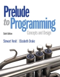
Transcribed Image Text:Markdown
O nbdiff l
123.771659
128.10434637 140.17173392 146.29001843 152.50565637
152.95840512]
Value of slope :
Value of intercept :
Value of uncertainity: 2.8384283514953754
3.0122239458296414
4.89877050906963
Q2B - Plotting 1
Plot the data from the previous question along with a trendline. Make sure to include proper labels on the axes, but you do not require a title or caption for this
plot.
In [183]: import matplotlib.pyplot as plt
import numpy as np
plt.figure(figsize=(8,4))
import matplotlib.pyplot as plt
import pandas as pd
from scipy.optimize import curve_fit
import numpy as np
samplex = np.linspace(e, 5e, 26) + np.random.normal(scale = 0.2, size = 26)
sampleY = 3 * samplex + 4 + np.random.normal (scale = 4, size = 26)
print(sampleY)
def obj(x,p,q) :
return p*x + q
ans1, ans2 = curve_fit(obj, samplex, sampleY)
P,q = ans1
print('Value of slope : ',p)
print('Value of intercept : ',q)
print('Value of uncertainity : ',np.sqrt(np.mean(np.power(sampley-(p*samplex +q),2))))
28.41670821
27.08235946
[ -0.71156319
21.20507976 19.03069129
O G 40)
ENG
(?
-19°C Clear
e to search
Chp
![Use the provided code to generate a dataset. Then, using a linear fitting routine to find the slope, intercept, and their uncertainties.
[9]: import matplotlib.pyplot as plt
import pandas as pd
import numpy as np
samplex = np.1linspace(0, 50, 26) + np.random.normal(scale = 0.2, size = 26)
sampleY = 3 * samplex + 4 + np.random.normal(scale = 4, size = 26)
print(sampleY)
[ -3.7460733
10.82831164
22.11521127
27.05865078
28.19418316
36.29761906
35.88279561
45.12991823 49.03624219
61.81609706
62.08941189
68.28062895
72.82874402
82.86838693 89.16999058
91.22403625
96.68730642 102.09560962 112.07930064 111.82978822
124.77577466 122.28792314 139.47251684 144.67256319 155.22459033
161.55767025]
In [24]:
import matplotlib.pyplot as plt
import pandas as pd
import numpy as np
samplex = np.linspace(0, 50, 26) + np.random.normal(scale = 0.2, size = 26)
sampleY = 3 * samplex + 4 + np.random.normal(scale = 4, size = 26)
print(sampleY)
plt.figure(figsize=(10,10))
#plt.plot(x,y,linestyle="-",linewidth=5,color="purple", Label="kinetic")
(?
-18°C Mostly cloudy
hp](/v2/_next/image?url=https%3A%2F%2Fcontent.bartleby.com%2Fqna-images%2Fquestion%2F44e7a3ce-803b-45aa-8658-f230b13e4980%2F9b3eb371-5b67-41cb-96d2-0c1fbbb6ab9f%2Ffd98pto_processed.jpeg&w=3840&q=75)
Transcribed Image Text:Use the provided code to generate a dataset. Then, using a linear fitting routine to find the slope, intercept, and their uncertainties.
[9]: import matplotlib.pyplot as plt
import pandas as pd
import numpy as np
samplex = np.1linspace(0, 50, 26) + np.random.normal(scale = 0.2, size = 26)
sampleY = 3 * samplex + 4 + np.random.normal(scale = 4, size = 26)
print(sampleY)
[ -3.7460733
10.82831164
22.11521127
27.05865078
28.19418316
36.29761906
35.88279561
45.12991823 49.03624219
61.81609706
62.08941189
68.28062895
72.82874402
82.86838693 89.16999058
91.22403625
96.68730642 102.09560962 112.07930064 111.82978822
124.77577466 122.28792314 139.47251684 144.67256319 155.22459033
161.55767025]
In [24]:
import matplotlib.pyplot as plt
import pandas as pd
import numpy as np
samplex = np.linspace(0, 50, 26) + np.random.normal(scale = 0.2, size = 26)
sampleY = 3 * samplex + 4 + np.random.normal(scale = 4, size = 26)
print(sampleY)
plt.figure(figsize=(10,10))
#plt.plot(x,y,linestyle="-",linewidth=5,color="purple", Label="kinetic")
(?
-18°C Mostly cloudy
hp
Expert Solution
This question has been solved!
Explore an expertly crafted, step-by-step solution for a thorough understanding of key concepts.

This is a popular solution!

Trending now
This is a popular solution!

Step by step
Solved in 4 steps with 2 images

Recommended textbooks for you
Computer Networking: A Top-Down Approach (7th Edi…
Computer Engineering
ISBN:
9780133594140
Author:
James Kurose, Keith Ross
Publisher:
PEARSON

Computer Organization and Design MIPS Edition, Fi…
Computer Engineering
ISBN:
9780124077263
Author:
David A. Patterson, John L. Hennessy
Publisher:
Elsevier Science

Network+ Guide to Networks (MindTap Course List)
Computer Engineering
ISBN:
9781337569330
Author:
Jill West, Tamara Dean, Jean Andrews
Publisher:
Cengage Learning
Computer Networking: A Top-Down Approach (7th Edi…
Computer Engineering
ISBN:
9780133594140
Author:
James Kurose, Keith Ross
Publisher:
PEARSON
Computer Organization and Design MIPS Edition, Fi…
Computer Engineering
ISBN:
9780124077263
Author:
David A. Patterson, John L. Hennessy
Publisher:
Elsevier Science
Network+ Guide to Networks (MindTap Course List)
Computer Engineering
ISBN:
9781337569330
Author:
Jill West, Tamara Dean, Jean Andrews
Publisher:
Cengage Learning
Concepts of Database Management
Computer Engineering
ISBN:
9781337093422
Author:
Joy L. Starks, Philip J. Pratt, Mary Z. Last
Publisher:
Cengage Learning
Prelude to Programming
Computer Engineering
ISBN:
9780133750423
Author:
VENIT, Stewart
Publisher:
Pearson Education

Sc Business Data Communications and Networking, T…
Computer Engineering
ISBN:
9781119368830
Author:
FITZGERALD
Publisher:
WILEY