![MATLAB: An Introduction with Applications](https://www.bartleby.com/isbn_cover_images/9781119256830/9781119256830_smallCoverImage.gif)
MATLAB: An Introduction with Applications
6th Edition
ISBN: 9781119256830
Author: Amos Gilat
Publisher: John Wiley & Sons Inc
expand_more
expand_more
format_list_bulleted
Question
![The figure below compares the share of global CO2 emissions vs. global share of population by
country for the year 2015. A line of parity is also indicated on the graph. Countries that lie on
this line account for the same share of global emissions as they do global population.
log10 (Percentage share of global CO₂ emissions)
H
2
~ m
Other countries
Australia
Parity line
-2
1
0
1
log10 (Percentage share of world population)
2
(c) Explain what it means for Australia to lie above the parity line in this figure.
(d) Explain the possible ramifications of using a global per capita average for CO2 emissions in
modelling Australian CO₂ emissions for the development of future energy policies.](https://content.bartleby.com/qna-images/question/44825f47-7947-4d58-9e56-09138ff3953c/05ac723a-ed94-4e95-ab48-4bfecf0ff93c/qn4bi7e_thumbnail.png)
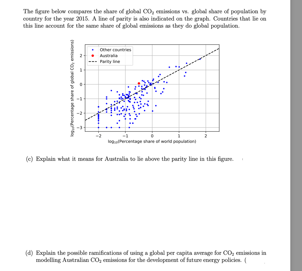
Transcribed Image Text:The figure below compares the share of global CO2 emissions vs. global share of population by
country for the year 2015. A line of parity is also indicated on the graph. Countries that lie on
this line account for the same share of global emissions as they do global population.
log10 (Percentage share of global CO₂ emissions)
H
2
~ m
Other countries
Australia
Parity line
-2
1
0
1
log10 (Percentage share of world population)
2
(c) Explain what it means for Australia to lie above the parity line in this figure.
(d) Explain the possible ramifications of using a global per capita average for CO2 emissions in
modelling Australian CO₂ emissions for the development of future energy policies.
Expert Solution
![Check Mark](/static/check-mark.png)
This question has been solved!
Explore an expertly crafted, step-by-step solution for a thorough understanding of key concepts.
Step by stepSolved in 4 steps
![Blurred answer](/static/blurred-answer.jpg)
Knowledge Booster
Similar questions
- 3. calculate these mortality rates: A) Crude mortality rate due to cancer B) Age specific mortality for adults age 55 and older C) The proportional mortality ratio (PMR) for cancer deathsarrow_forwardTABLE 8.1 2016 Marginal Tax Rates, Standard Deductions, and Exemptions Unmaried, diverced, or legally separated Married and ach parteer files eparate tar rete Married and berh partren file single tar retee Unmarried and paying mare than half the cest of sepperting ekildr pareet Married Filing Separately Married Filing Jointly Head of Household Тах Rate Single 10% up to $9275 up to $9275 up to $18,550 up to $13.250 15% $9276 to $37,650 $9276 to $37,650 $18,551 to $75,300 $13,251 to $50,400 25% $37,651 to $91,150 $37,651 to $75,950 $75,301 to $151,900 $50,401 to $130,150 28% $91,151 to $190,150 S75,951 to $115,725 $151,901 to $231,450 $130,151 to $210,800 33% $190,151 to $413,350 SI15,726 to $206,675 $231,451 to $413,350 $210,801 to $413,350 35% $413,351 to $415,050 $206,676 to $233,475 $413,351 to $466,950 $413,351 to $441,000 39.6% mure than $441,000 more than S415.050 more than $233.475 mure than $466,950 Standard Deduction $6300 $600 $12,600 $9300 Exemptions (per person) $4050 S4050…arrow_forwardConsider the following. March April May Month Demand. January 29 February March June April July May June July What is the forecast for July based on a three-month weighted moving average applied to the above past demand data and using the weights: data)? Show all the forecasts for April through June along with the answer Month Demand Forecast January 29 February 46 58 59 46 74 58 59 = 74 88 53 10 10 1:35:14 and (largest weight is for most recent 10arrow_forward
- Exercise 2. Use the final project data to complete the following questions. Collaborate with your project partners and produce the Excel outputs for the first analysis listed on the project guidelines below. Read and follow the instructions carefully. The Excel outputs such as tables, graphs, summary statistics produced by using Excel. All statistics should not have more than 2 decimal places. All Excel outputs (such as graphs and summary statistics) for each related analysis must be fitted in one sheet. 2. To analyze the total number of items purchased, construct an ungrouped frequency distribution, graph, and find the summary statistics by each type of customer (regular/promotion). Label the graphs completely. Describe the shape of the distribution for each type of customer and discuss similarities or differences by interpreting the graphs and summary statistics. What can you conclude? 3. To analyze customer age, construct a frequency distribution, graph, and find…arrow_forwardTable 1. The manager of Carpet City outlet store needs to be able to forecast accurately demand for Soft Shang carpet. Demand for the past 20 weeks appears in table 1 below. week Demand Forecast Error ABS. Dev Squared Error APE 1 20 2 28 3 22 4 18 5 22 6 22 7 22 8 26 9 23 10 23 11 23 12 27 13 25 14 22 15 23 16 14 17 14 18 15 19 11 20 16 21 22 23 24…arrow_forwardThe Organization for Economic Cooperation and Development (OECD) consists of 20 industrialized countries. For these nations, the prediction equation relating y = child poverty rate (in percentage points) to x = social expenditure as a percentage of gross domestic product (GDP) is = 22-1.3x. In 2000, the actual child poverty rate ranged from 2.8% (in Finland) to 21.9% (in the U.S.). Social expenditure as a percentage of GDP ranged from 2% (in the United States) to 16% (in Denmark). What is the value of the y-intercept (a) estimated in the linear prediction equation provided above (= 22-1.3x)? Also, interpret the y-intercept. y-intercept: Interpretation of y-intercept:arrow_forward
- 2. A town has a population of 8400 in the year 1990. Fifteen years later, its population grew to 12,500. A) Determine the growth rate of this town's population. B) Predict the population in the town in the year 2050. C) In which year would the town's population be just above 20,000? D) If this model were valid until only the year 2090, determine the domain and range of this model.arrow_forward7. Calculate the weighted price index from the following data : Quantity required Price during 1995 Materia! Unit 1994 i required 2$ $ 8.0 Cement Timber Steel sheet: Bricks 500 lb. 2,000 c.ft. 50 cwt. 5.0 9.5 100 lb. c.ft. 14.2 34.0 12.0 cwt. 42.0 per '000 20,000 24.0arrow_forwardQUESTIONS ARE:1.Using linear regression analysis, the estimated variable cost per labor hour for maintenance is closest to2.Refer to Paul Company. Using linear regression analysis, the estimated fixed cost per month for maintenance is closest to3.Refer to Paul Company. Based upon the data derived from the regression analysis, 450 maintenance hours in a month would mean the maintenance costs (rounded to the nearest peso) would be budgeted atarrow_forward
arrow_back_ios
arrow_forward_ios
Recommended textbooks for you
- MATLAB: An Introduction with ApplicationsStatisticsISBN:9781119256830Author:Amos GilatPublisher:John Wiley & Sons IncProbability and Statistics for Engineering and th...StatisticsISBN:9781305251809Author:Jay L. DevorePublisher:Cengage LearningStatistics for The Behavioral Sciences (MindTap C...StatisticsISBN:9781305504912Author:Frederick J Gravetter, Larry B. WallnauPublisher:Cengage Learning
- Elementary Statistics: Picturing the World (7th E...StatisticsISBN:9780134683416Author:Ron Larson, Betsy FarberPublisher:PEARSONThe Basic Practice of StatisticsStatisticsISBN:9781319042578Author:David S. Moore, William I. Notz, Michael A. FlignerPublisher:W. H. FreemanIntroduction to the Practice of StatisticsStatisticsISBN:9781319013387Author:David S. Moore, George P. McCabe, Bruce A. CraigPublisher:W. H. Freeman
![Text book image](https://www.bartleby.com/isbn_cover_images/9781119256830/9781119256830_smallCoverImage.gif)
MATLAB: An Introduction with Applications
Statistics
ISBN:9781119256830
Author:Amos Gilat
Publisher:John Wiley & Sons Inc
![Text book image](https://www.bartleby.com/isbn_cover_images/9781305251809/9781305251809_smallCoverImage.gif)
Probability and Statistics for Engineering and th...
Statistics
ISBN:9781305251809
Author:Jay L. Devore
Publisher:Cengage Learning
![Text book image](https://www.bartleby.com/isbn_cover_images/9781305504912/9781305504912_smallCoverImage.gif)
Statistics for The Behavioral Sciences (MindTap C...
Statistics
ISBN:9781305504912
Author:Frederick J Gravetter, Larry B. Wallnau
Publisher:Cengage Learning
![Text book image](https://www.bartleby.com/isbn_cover_images/9780134683416/9780134683416_smallCoverImage.gif)
Elementary Statistics: Picturing the World (7th E...
Statistics
ISBN:9780134683416
Author:Ron Larson, Betsy Farber
Publisher:PEARSON
![Text book image](https://www.bartleby.com/isbn_cover_images/9781319042578/9781319042578_smallCoverImage.gif)
The Basic Practice of Statistics
Statistics
ISBN:9781319042578
Author:David S. Moore, William I. Notz, Michael A. Fligner
Publisher:W. H. Freeman
![Text book image](https://www.bartleby.com/isbn_cover_images/9781319013387/9781319013387_smallCoverImage.gif)
Introduction to the Practice of Statistics
Statistics
ISBN:9781319013387
Author:David S. Moore, George P. McCabe, Bruce A. Craig
Publisher:W. H. Freeman