! = 1.89 – 1.25 = 0.64 = (0.8) 5.13 – 1.89 = 3.24 = (1.8)´ 5.94 – 5.13 = 0.81=(0.9)´ 9.18 – 5.94 = 3.24 = (1.8)´ * 12.42 –9.18 = 3.24 = (1.8) 1.25 + (0.8)* + (1.8) +(0.9) +(1.8)* + (1.8)*


Contingency Table
A contingency table can be defined as the visual representation of the relationship between two or more categorical variables that can be evaluated and registered. It is a categorical version of the scatterplot, which is used to investigate the linear relationship between two variables. A contingency table is indeed a type of frequency distribution table that displays two variables at the same time.
Binomial Distribution
Binomial is an algebraic expression of the sum or the difference of two terms. Before knowing about binomial distribution, we must know about the binomial theorem.
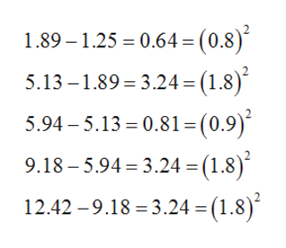
- A pet store offered a baby monkey for sale at $1.25. The monkey grew, and the next week it was offered at $1.89. Not one to monkey around, the shopkeeper subsequently raised the price to $5.13, then to $5.94, and next to $9.18. Finally, during the sixth week, an organ grinder bought the monkey at $12.42. How were the prices figured?
- The amount of baby monkey is $1.25; the next week it is offered at $1.89.
- Then, raised to $5.13, then raised to $5.94, next to $9.18. Finally, the sixth week the amount at which it was sold is $12.42.
- Find the differences between the digits as follows:
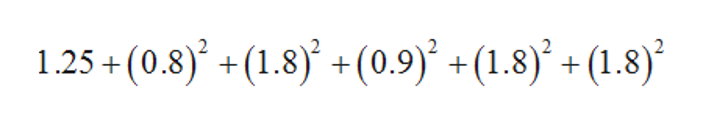
The sequence obtained starting from $1.25 is
As the pattern is not obtained, it can be assumed that there is some unfixed rate which is squared and added to each week price.
Thus, the prices are figured in an uneven manner.


Trending now
This is a popular solution!

Step by step
Solved in 4 steps with 1 images


