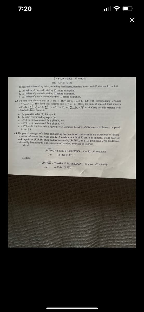
Please answer a-f for 4.4 7:20y=64.29 +0.99x R0.379(se) (2.42) (0.18)Rewrite the estimated equation, including coefficients, standard errors, and R², that would result ifa. All values of x were divided by 10 before estimation.b. All values of y were divided by 10 before estimation.c. All values of y and x were divided by 10 before estimation.4.3 We have five observations on x and y. They are x = 3, 2, 1,-1,0 with corresponding y values1.2 +0.8x,, the sum of squared least squares(y,-5)= 10. Carry out this exercise withy = 4,2,3,1,0. The fitted least squares line is ŷ,residuals is = 3.6,a hand calculator. Compute(x-7)= 10, anda. the predicted value of y for x, 4.b. the se) corresponding to part (a).c. a 95% prediction interval for y given x = 4.d. a 99% prediction interval for y given.x = 4.e. a 95% prediction interval for y given.x = 7. Compare the width of this interval to the one computedin part (c).4.4 The general manager of a large engineering firm wants to know whether the experience of techni-cal artists influences their work quality. A random sample of 50 artists is selected. Using years ofwork experience (EXPER) and a performance rating (RATING, on a 100-point scale), two models areestimated by least squares. The estimates and standard errors are as follows:Model 1:Model 2:RATING= 64.289 +0.990EXPER N=50 R²=0.3793(se)(2.422) (0.183)RATING= 39.464+15.312 In(EXPER) N=46 R = 0.6414(se) (4.198) (1.727) 7:21Prediction, Goodness-of-Fit, and Modeling Issuesa. Sketch the fitted values from Model 1 for EXPER=0 to 30 years.b. Sketch the fitted values from Model 2 against EXPER= 1 to 30 years. Explain why the four artistswith no experience are not used in the estimation of Model 2.c. Using Model 1, compute the marginal effect on RATING of another year of experience for (i) anartist with 10 years of experience and (ii) an artist with 20 years of experience.d. Using Model 2, compute the marginal effect on RATING of another year of experience for (i) anartist with 10 years of experience and (ii) an artist with 20 years of experience.e. Which of the two models fits the data better? Estimation of Model 1 using just the technical artistswith some experience yields R² = 0.4858.f. Do you find Model 1 or Model 2 more reasonable, or plausible, based on economic reasoning?Explain.4.5 Consider the regression model WAGE=B₁ + BEDUC+ e. WAGE is hourly wage rate in U.S. 2013dollars. EDUC is years of education attainment, or schooling. The model is estimated using individu-als from an urban area.WAGE= -10.76+2.461965EDUC, N=986(2.27) (0.16)(se)a. The sample standard deviation of WAGE is 15.96 and the sum of squared residuals from the regres-sion above is 199,705.37. Compute R².b. Using the answer to (a), what is the correlation between WAGE and EDUC? [Hint: What is thecorrelation between WAGE and the fitted value WAGE?]c. The sample mean and variance of EDUC are 14.315 and 8.555, respectively. Calculate the leverageof observations with EDUC=5, 16, and 21. Should any of the values be considered large?d. Omitting the ninth observation, a person with 21 years of education and wage rate $30.76, andreestimating the model we find = 14.25 and an estimated slope of 2.470095. Calculate DFBETASfor this observation. Should it be considered large?e. For the ninth observation, used in part (d), DFFITS = -0.0571607. Is this value large? The leveragevalue for this observation was found in part (c). How much does the fitted value for this observationchange when this observation is deleted from the sample?f. For the ninth observation, used in parts (d) and (e), the least squares residual is -10late the studentized residual. Should it be considered large?of squareiha hand.4.6 We have five observations on x and y. They are x, = 3,2,1,-1,0 with correspo10. The fitted least squares line is= 1.2+0.8x,. the10. Carry out this ex

Question

Accepted Answer

Given,
Model 1 : 
RATING^se=64.2892.422+0.9900.183EXPER   N=50   R2=0.3793
Model 2 :…