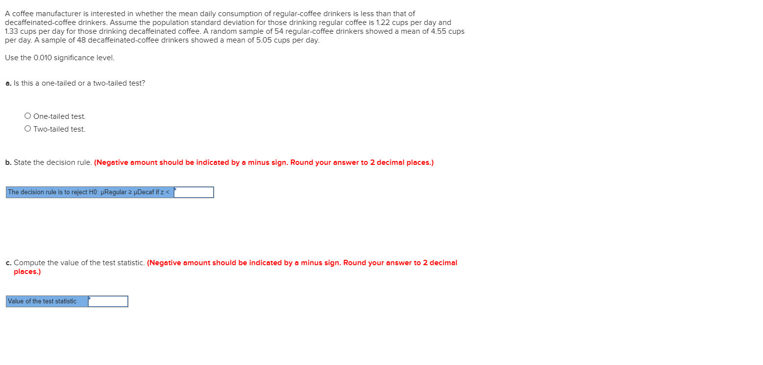
A coffee manufacturer is interested in whether the mean daily consumption of regular-coffee drinkers is less than that of decaffeinated-coffee drinkers. Assume the population standard deviation for those drinking regular coffee is 1.22 cups per day and 1.33 cups per day for those drinking decaffeinated coffee. A random sample of 54 regular-coffee drinkers showed a mean of 4.55 cups per day. A sample of 48 decaffeinated-coffee drinkers showed a mean of 5.05 cups per day. Use the 0.010 significance level. a. Is this a one-tailed or a two-tailed test? O One-tailed test. O Two-tailed test. b. State the decision rule. (Negative amount should be indicated by a minus sign. Round your answer to 2 decimal places.) The decision rule is to reject H0: µRegular 2 µDecaf if z < c. Compute the value of the test statistic. (Negative amount should be indicated by a minus sign. Round your answer to 2 decimal places.) Value of the test statistic

Bone mineral density (BMD) is a measure of bone strength. Studies show that BMD declines after age 45. The impact of exercise may increase BMD. A random sample of 59 women between the ages of 41 and 45 with no major health problems were studied. The women were classified into one of two groups based upon their level of exercise activity: walking women and sedentary women. The 39 women who walked regularly had a mean BMD of 5.96 with a standard deviation of 1.22. The 20 women who are sedentary had a mean BMD of 4.41 with a standard deviation of 1.02. Which of the following inference procedures could be used to estimate the difference in the mean BMD for these two types of women

The heights of 10 year old American children are normally distributed with a mean height of 4 feet and 5 inches (or 53 inches) and a standard deviation of 4.5 inches.In order to be allowed to go on a particular kids ride at the amusement park, children must be at least 44.9 inches tall and no more than 59.75 inches tall.What percent of 10 year old American children cannot go on the ride?

According to Kaiser Family Foundation survey in 2011 and 2010, the average premium for employer-sponsored health insurance for family coverage was $15,073 in 2011 and $13,770 in 2010 (USA TODAY, September 29, 2011). Suppose that these averages were based on random samples of 250 and 200 employees who had such employer-sponsored health insurance plans for 2011 and 2010, respectively. Further assume that the population standard deviations for 2011 and 2010 were $2160 and $1990, respectively.

In a sample of 351 gamers between the ages of 16-25, the mean number of hours spent gaming per week was 42.5 hours. In a sample of 269 gamers between the ages of 26-40, the mean number of hours spent gaming per week was 43.8 hours. If the population standard deviation for the mean number of hours spent gaming per week is 9.5 for the age group 16-25 and 10.7 for the age group 26-40, test the claim that gamers between the ages of 16-25 spend less time gaming per week than gamers between the ages of 26-40. Assume α=0.03.      Let population 1 be gamers in the age group 16-25 and population 2 be gamers in the age group 26-40. Round the test statistic to two decimal places, and round the p-value to four decimal places.   The test statistic is . The p-value is . Should the null hypothesis be rejected?

The combined SAT scores for the students at a local high school are normally distributed with a mean of 1469 and a standard deviation of 296. The local college includes a minimum score of 1824 in its admission requirements. What percentage of students from this school earn scores that satisfy the admission requirement?

Help

Steve believes that his wife's cell phone battery does not last as long as his cell phone battery. On eight different occasions, he measured the length of time his cell phone battery lasted and calculated that the mean was 19.7 hours with a standard deviation of 9.4 hours. He measured the length of time his wife's cell phone battery lasted on twelve different occasions and calculated a mean of 18.9 hours with a standard deviation of 5.3 hours. Assume that the population variances are the same. Let Population 1 be the battery life of Steve's cell phone and Population 2 be the battery life of his wife's cell phone. Step 1 of 2: Construct a 90 % confidence interval for the true difference in mean battery life between Steve's cell phone and his wife's. Round the endpoints of the interval to one decimal place, if necessary.

A research article reported that for a random sample of 850 meal purchases made at fast food chain A, the mean number of calories was 1,004, and the standard deviation was 489. For a random sample of 2,108 meal purchases made at fast food chain B, the mean number of calories was 905, and the standard deviation was 622. Based on these samples, is there convincing evidence that the mean number of calories in fast food chain B meal purchases is less than the mean number of calories in fast food chain A meal purchases? (Test the relevant hypotheses using a 0.05 level of significance. Use ?1 for fast food chain B and ?2 for fast food chain A.)   State the appropriate null and alternative hypotheses.   Find the test statistic and P-value. (Use SALT. Round your test statistic to one decimal place and your P-value to three decimal places.) t= P-value=   State the conclusion in the problem context. We fail to reject H0. There is convincing evidence that the mean number of calories in fast food…

A car company claims that its new SUV gets better gas mileage than its competitor's SUV. A random sample of 41 of its SUVs has a mean gas mileage of 15.2 miles per gallon (mpg). The population standard deviation is known to be 1.4 mpg. A random sample of 49 competitor's SUVs has a mean gas mileage of 14.8 mpg. The population standard deviation for the competitor is known to be 0.9 mpg. Test the company's claim at the 0.02 level of significance. Let the car company's SUVs be Population 1 and let the competitor's SUVs be Population 2. Step 1 of 3: State the null and alternative hypotheses for the test. Fill in the blank below. Ho:μ₁ = μ₂ Ha : M 1₂