A random sample of 46 adult coyotes in a region of northern Minnesota showed the average age to be x = 2.03 years, with sample standard deviations = 0.76 years. However, it is thought that the overall population mean age of coyotes is = 1.75. Do the sample data indicate that coyotes in this region of northern Minnesota tend to live longer than the average of 1.75 years? Use a = 0.01. USE SALT (a) What is the level of significance? State the null and alternate hypotheses. Ho: < 1.75 yr; H₁: = 1.75 yr O Ho: > 1.75 yr; H₁: = 1.75 yr O Ho: = 1.75 yr; H₁: > 1.75 yr Ho: = 1.75 yr; H₁: < 1.75 yr O Ho: = 1.75 yr; H₁: ## 1.75 yr (b) What sampling distribution will you use? Explain the rationale for your choice of sampling distribution. O The Student's t, since the sample size is large and o is unknown. O The standard normal, since the sample size is large and o is known. O The standard normal, since the sample size is large and o is unknown. O The Student's t, since the sample size is large and a is known. What the of the sampl (c) Estimate the P-value. OP-value> 0.250 O 0.100 < P-value < 0.250 O 0.050 < P-value < 0.100. O 0.010 P-value < 0.050 OP-value < 0.010 statistic? (Round your answer to three ces.)
A random sample of 46 adult coyotes in a region of northern Minnesota showed the average age to be x = 2.03 years, with sample standard deviations = 0.76 years. However, it is thought that the overall population mean age of coyotes is = 1.75. Do the sample data indicate that coyotes in this region of northern Minnesota tend to live longer than the average of 1.75 years? Use a = 0.01. USE SALT (a) What is the level of significance? State the null and alternate hypotheses. Ho: < 1.75 yr; H₁: = 1.75 yr O Ho: > 1.75 yr; H₁: = 1.75 yr O Ho: = 1.75 yr; H₁: > 1.75 yr Ho: = 1.75 yr; H₁: < 1.75 yr O Ho: = 1.75 yr; H₁: ## 1.75 yr (b) What sampling distribution will you use? Explain the rationale for your choice of sampling distribution. O The Student's t, since the sample size is large and o is unknown. O The standard normal, since the sample size is large and o is known. O The standard normal, since the sample size is large and o is unknown. O The Student's t, since the sample size is large and a is known. What the of the sampl (c) Estimate the P-value. OP-value> 0.250 O 0.100 < P-value < 0.250 O 0.050 < P-value < 0.100. O 0.010 P-value < 0.050 OP-value < 0.010 statistic? (Round your answer to three ces.)

MATLAB: An Introduction with Applications
6th Edition
ISBN:9781119256830
Author:Amos Gilat
Publisher:Amos Gilat
Chapter1: Starting With Matlab
Section: Chapter Questions
Problem 1P

Related questions
Question
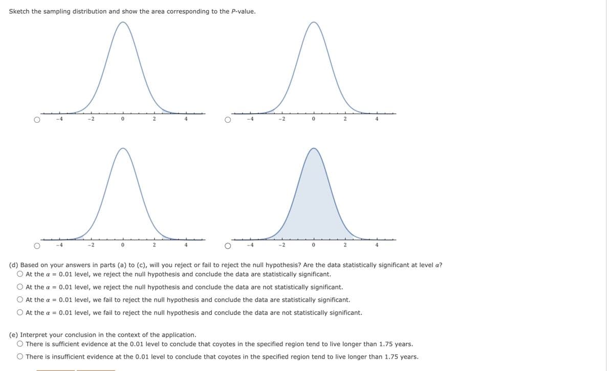
Transcribed Image Text:Sketch the sampling distribution and show the area corresponding to the P-value.
^ ^
0
2
0
-4
-2
0
-4
-4
-2
0
2
2
(d) Based on your answers in parts (a) to (c), will you reject or fail to reject the null hypothesis? Are the data statistically significant at level a?
O At the a = 0.01 level, we reject the null hypothesis and conclude the data are statistically significant.
O At the a = 0.01 level, we reject the null hypothesis and conclude the data are not statistically significant.
O At the a = 0.01 level, we fail to reject the null hypothesis and conclude the data are statistically significant.
O At the a = 0.01 level, we fail to reject the null hypothesis and conclude the data are not statistically significant.
(e) Interpret your conclusion in the context of the application.
O There is sufficient evidence at the 0.01 level to conclude that coyotes in the specified region tend to live longer than 1.75 years.
O There is insufficient evidence at the 0.01 level to conclude that coyotes in the specified region tend to live longer than 1.75 years.
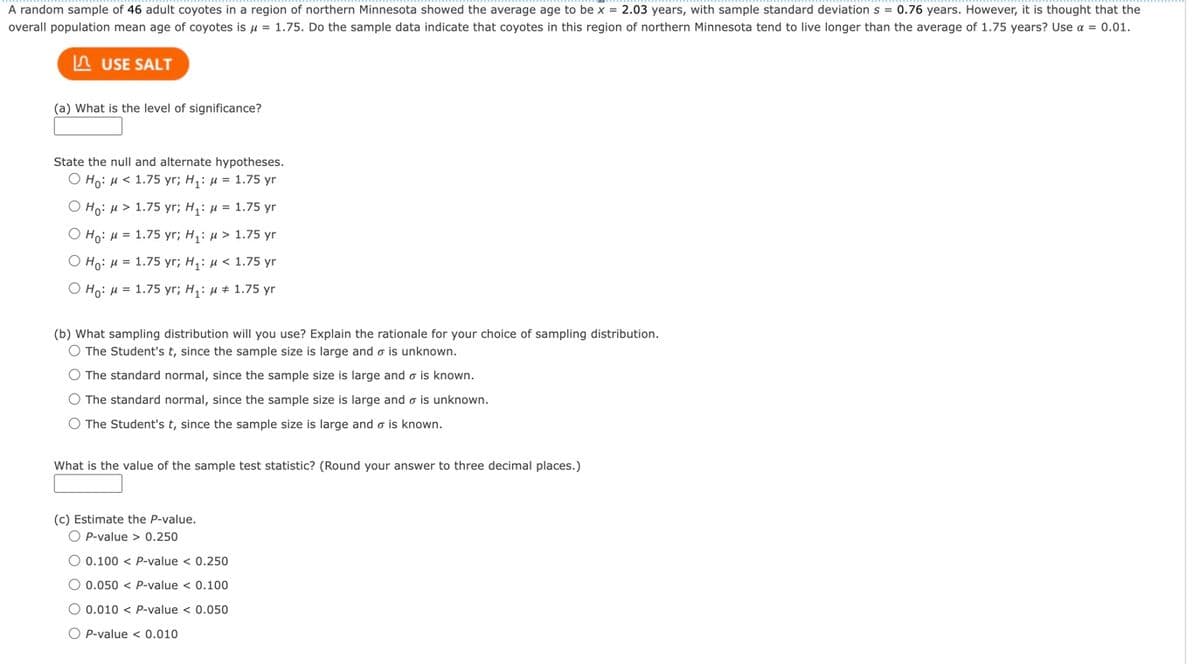
Transcribed Image Text:A random sample of 46 adult coyotes in a region of northern Minnesota showed the average age to be x = 2.03 years, with sample standard deviation s = 0.76 years. However, it is thought that the
overall population mean age of coyotes is μ = 1.75. Do the sample data indicate that coyotes in this region of northern Minnesota tend to live longer than the average of 1.75 years? Use a = 0.01.
USE SALT
(a) What is the level of significance?
State the null and alternate hypotheses.
O Ho: μ< 1.75 yr; H₁: μ = 1.75 yr
O Ho: μ> 1.75 yr; H₁: μ = 1.75 yr
O Ho: μ =
1.75 yr; H₁: μ> 1.75 yr
O Ho: μ = 1.75 yr; H₁: μ< 1.75 yr
O Ho: μ = 1.75 yr; H₁:
1.75 yr
(b) What sampling distribution will you use? Explain the rationale for your choice of sampling distribution.
O The Student's t, since the sample size is large and o is unknown.
O The standard normal, since the sample size is large and o is known.
O The standard normal, since the sample size is large and o is unknown.
O The Student's t, since the sample size is large and o is known.
What is the value of the sample test statistic? (Round your answer to three decimal places.)
(c) Estimate the P-value.
OP-value > 0.250
O 0.100 < P-value < 0.250
O 0.050 < P-value < 0.100
O 0.010 < P-value < 0.050
O P-value < 0.010
Expert Solution
This question has been solved!
Explore an expertly crafted, step-by-step solution for a thorough understanding of key concepts.

Step by step
Solved in 5 steps

Recommended textbooks for you
MATLAB: An Introduction with Applications
Statistics
ISBN:
9781119256830
Author:
Amos Gilat
Publisher:
John Wiley & Sons Inc

Probability and Statistics for Engineering and th…
Statistics
ISBN:
9781305251809
Author:
Jay L. Devore
Publisher:
Cengage Learning

Statistics for The Behavioral Sciences (MindTap C…
Statistics
ISBN:
9781305504912
Author:
Frederick J Gravetter, Larry B. Wallnau
Publisher:
Cengage Learning
MATLAB: An Introduction with Applications
Statistics
ISBN:
9781119256830
Author:
Amos Gilat
Publisher:
John Wiley & Sons Inc
Probability and Statistics for Engineering and th…
Statistics
ISBN:
9781305251809
Author:
Jay L. Devore
Publisher:
Cengage Learning
Statistics for The Behavioral Sciences (MindTap C…
Statistics
ISBN:
9781305504912
Author:
Frederick J Gravetter, Larry B. Wallnau
Publisher:
Cengage Learning

Elementary Statistics: Picturing the World (7th E…
Statistics
ISBN:
9780134683416
Author:
Ron Larson, Betsy Farber
Publisher:
PEARSON

The Basic Practice of Statistics
Statistics
ISBN:
9781319042578
Author:
David S. Moore, William I. Notz, Michael A. Fligner
Publisher:
W. H. Freeman

Introduction to the Practice of Statistics
Statistics
ISBN:
9781319013387
Author:
David S. Moore, George P. McCabe, Bruce A. Craig
Publisher:
W. H. Freeman