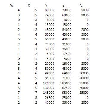
A researcher wants to determine the causal relationship among number of family members who are at least high school graduate (W), number of working family members (X), monthly gross income (Y), monthly expenditure (Z), and average monthly bank deposits (A). A random sample of 20 families was selected and the data on the variables were collected (see household.xslx). Consider the following path diagram: 1. Set-up the structural equations. Consider the R outputs from the conducted path analysis.


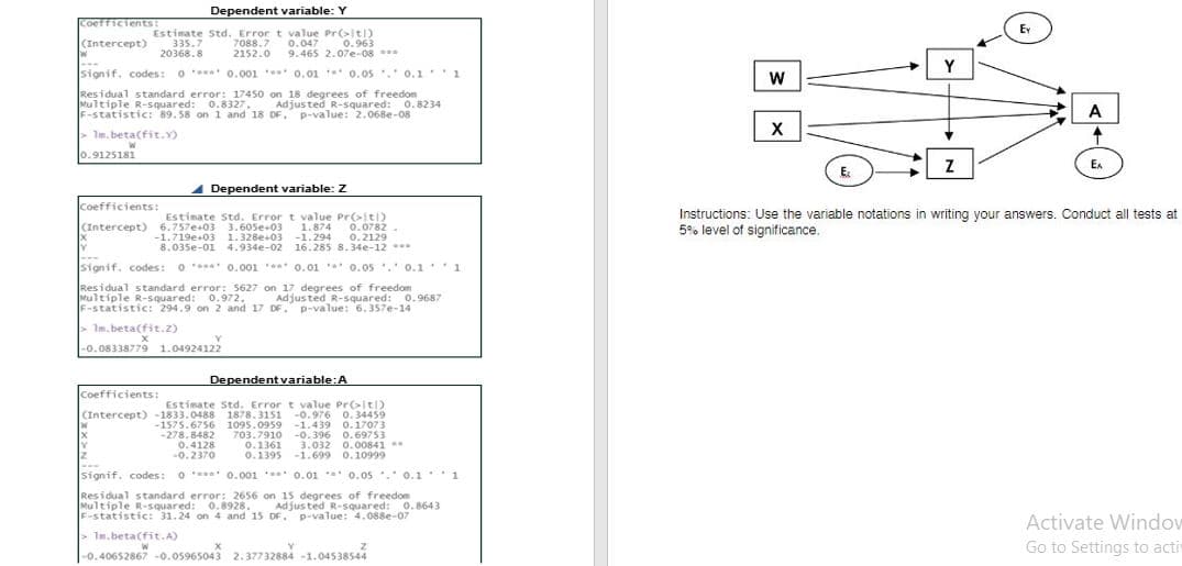
A researcher wants to determine the causal relationship among number of family members who are at least high school graduate (W), number of working family members (X), monthly gross income (Y), monthly expenditure (Z), and average monthly bank deposits (A). A random sample of 20 families was selected and the data on the variables were collected (see household.xslx). Consider the following path diagram:
1. Set-up the structural equations. Consider the R outputs from the conducted path analysis.
2. Identify the factors affecting the endogenous variables. Leave blank if variable is exogenous.
W: ____________
X: ____________
Y: ____________
Z: ____________
A: ____________
3. Illustrate the output path diagram including the estimated path coefficients.

Step by step
Solved in 4 steps with 4 images

