(a) There are 97% of the cars will be loaded with more than K tons of coal. What is the value of K? (b) What is the probability that one car chosen at random will have less than 74.4 tons of coal? (c) Among 20 randomly chosen cars, what is the probability that more than 2 cars will be loaded with less than 74.4 tons of coal?

MATLAB: An Introduction with Applications
6th Edition
ISBN:9781119256830
Author:Amos Gilat
Publisher:Amos Gilat
Chapter1: Starting With Matlab
Section: Chapter Questions
Problem 1P
icon
Related questions
Question

Coal is carried from a mine in West Virginia to a power plant in New York in hopper cars on a long train. The
automatic hopper car loader is set to put 75 tons of coal into each car. The actual weight of coal loaded into
each car is normally distributed, with mean of 75 tons and standard deviation of 0.8 ton.


(a) There are 97% of the cars will be loaded with more than K tons of coal. What is the value of K?


(b) What is the probability that one car chosen at random will have less than 74.4 tons of coal?


(c) Among 20 randomly chosen cars, what is the probability that more than 2 cars will be loaded with less
than 74.4 tons of coal?


(d) Among 20 randomly chosen cars, most likely, how many cars will be loaded with less than 74.4 tons of
coal? Calculate the corresponding probability.


(e) In the senior management meeting, it is discussed and agreed that a car loaded with less than 74.4 tons
of coal is not cost effective. To reduce the ratio of cars to be loaded with less than 74.4 tons of coal, it
is suggested changing current average loading of coal from 75 tons to a new average level, M tons.
Should the new level M be (I) higher than 75 tons or (II) lower than 75 tons? (Write down your
suggestion, no explanation is needed in part (e)).
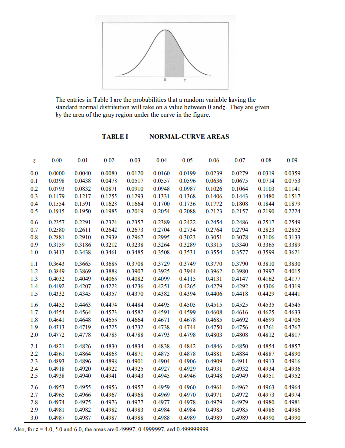
The entries in Table I are the probabilities that a random variable having the
standard normal distribution will take on a value between 0 andz. They are given
by the area of the gray region under the curve in the figure.
TABLE I
NORMAL-CURVE AREAS
0.00
0.01
0.02
0.03
0.04
0.05
0.06
0.07
0.08
0.09
0.0
0.0000
0.0040
0.0080
0.0120
0.0160
0.0199
0.0239
0.0279
0.0319
0.0359
0.1
0.0398
0.0438
0.0478
0.0517
0.0557
0.0596
0.0636
0.0675
0.0714
0.0753
0.2
0.0793
0.0832
0.0871
0.0910
0.0948
0.0987
0.1026
0.1064
0.1103
0.1141
0.3
0.1179
0.1217
0.1255
0.1293
0.1331
0.1368
0.1406
0.1443
0.1480
0.1517
0.4
0.1554
0.1591
0.1628
0.1664
0.1700
0.1736
0.1772
0.1808
0.1844
0.1879
0.5
0.1915
0.1950
0.1985
0.2019
0.2054
0.2088
0.2123
0.2157
0.2190
0.2224
0.6
0.2257
0.2291
0.2324
0.2357
0.2389
0.2422
0.2454
0.2486
0.2517
0.2549
0.7
0.2580
0.2611
0.2642
0.2673
0.2704
0.2734
0.2764
0.2794
0.2823
0.2852
0.8
0.2881
0.2910
0.2939
0.2967
0.2995
0.3023
0.3051
0.3078
0.3106
0.3133
0.9
0.3159
0.3186
0.3212
0.3238
0.3264
0.3289
0.3315
0.3340
0.3365
0.3389
1.0
0.3413
0.3438
0.3461
0.3485
0.3508
0.3531
0.3554
0.3577
0.3599
0.3621
1.1
0.3643
0.3665
0.3686
0.3708
0.3729
0.3749
0.3770
0.3790
0.3810
0.3830
1.2
0.3849
0.3869
0.3888
0.3907
0.3925
0.3944
0.3962
0.3980
0.3997
0.4015
1.3
0.4032
0.4049
0.4066
0.4082
0.4099
0.4115
0.4131
0.4147
0.4162
0.4177
1.4
0.4192
0.4207
0.4222
0.4236
0.4251
0.4265
0.4279
0.4292
0.4306
0.4319
1.5
0.4332
0.4345
0.4357
0.4370
0.4382
0.4394
0.4406
0.4418
0.4429
0.4441
1.6
0.4452
0.4463
0.4474
0.4484
0.4495
0.4505
0.4515
0.4525
0.4535
0.4545
1.7
0.4554
0.4564
0.4573
0.4582
0.4591
0.4599
0.4608
0.4616
0.4625
0.4633
1.8
0.4641
0.4648
0.4656
0.4664
0.4671
0.4678
0.4685
0.4692
0.4699
0.4706
1.9
0.4713
0.4719
0.4725
0.4732
0.4738
0.4744
0.4750
0.4756
0.4761
0.4767
2.0
0.4772
0.4778
0.4783
0.4788
0.4793
0.4798
0.4803
0.4808
0.4812
0.4817
2.1
0.4821
0.4826
0.4830
0.4834
0.4838
0.4842
0.4846
0.4850
0.4854
0.4857
2.2
0.4861
0.4864
0.4868
0.4871
0.4875
0.4878
0.4881
0.4884
0.4887
0.4890
2.3
0.4893
0.4896
0.4898
0.4901
0.4904
0.4906
0.4909
0.4911
0.4913
0.4916
2.4
0.4918
0.4920
0.4922
0.4925
0.4927
0.4929
0.4931
0.4932
0.4934
0.4936
2.5
0.4938
0.4940
0.4941
0.4943
0.4945
0.4946
0.4948
0.4949
0.4951
0.4952
2.6
0.4953
0.4955
0.4956
0.4957
0.4959
0.4960
0.4961
0.4962
0.4963
0.4964
2.7
0.4965
0.4966
0.4967
0.4968
0.4969
0.4970
0.4971
0.4972
0.4973
0.4974
2.8
0.4974
0.4975
0.4976
0.4977
0.4977
0.4978
0.4979
0.4979
0.4980
0.4981
2.9
0.4981
0.4982
0.4982
0.4983
0.4984
0.4984
0.4985
0.4985
0.4986
0.4986
3.0
0.4987
0.4987
0.4987
0.4988
0.4988
0.4989
0.4989
0.4989
0.4990
0.4990
Also, for z = 4.0, 5.0 and 6.0, the areas are 0.49997, 0.4999997, and 0.499999999.
Transcribed Image Text:The entries in Table I are the probabilities that a random variable having the standard normal distribution will take on a value between 0 andz. They are given by the area of the gray region under the curve in the figure. TABLE I NORMAL-CURVE AREAS 0.00 0.01 0.02 0.03 0.04 0.05 0.06 0.07 0.08 0.09 0.0 0.0000 0.0040 0.0080 0.0120 0.0160 0.0199 0.0239 0.0279 0.0319 0.0359 0.1 0.0398 0.0438 0.0478 0.0517 0.0557 0.0596 0.0636 0.0675 0.0714 0.0753 0.2 0.0793 0.0832 0.0871 0.0910 0.0948 0.0987 0.1026 0.1064 0.1103 0.1141 0.3 0.1179 0.1217 0.1255 0.1293 0.1331 0.1368 0.1406 0.1443 0.1480 0.1517 0.4 0.1554 0.1591 0.1628 0.1664 0.1700 0.1736 0.1772 0.1808 0.1844 0.1879 0.5 0.1915 0.1950 0.1985 0.2019 0.2054 0.2088 0.2123 0.2157 0.2190 0.2224 0.6 0.2257 0.2291 0.2324 0.2357 0.2389 0.2422 0.2454 0.2486 0.2517 0.2549 0.7 0.2580 0.2611 0.2642 0.2673 0.2704 0.2734 0.2764 0.2794 0.2823 0.2852 0.8 0.2881 0.2910 0.2939 0.2967 0.2995 0.3023 0.3051 0.3078 0.3106 0.3133 0.9 0.3159 0.3186 0.3212 0.3238 0.3264 0.3289 0.3315 0.3340 0.3365 0.3389 1.0 0.3413 0.3438 0.3461 0.3485 0.3508 0.3531 0.3554 0.3577 0.3599 0.3621 1.1 0.3643 0.3665 0.3686 0.3708 0.3729 0.3749 0.3770 0.3790 0.3810 0.3830 1.2 0.3849 0.3869 0.3888 0.3907 0.3925 0.3944 0.3962 0.3980 0.3997 0.4015 1.3 0.4032 0.4049 0.4066 0.4082 0.4099 0.4115 0.4131 0.4147 0.4162 0.4177 1.4 0.4192 0.4207 0.4222 0.4236 0.4251 0.4265 0.4279 0.4292 0.4306 0.4319 1.5 0.4332 0.4345 0.4357 0.4370 0.4382 0.4394 0.4406 0.4418 0.4429 0.4441 1.6 0.4452 0.4463 0.4474 0.4484 0.4495 0.4505 0.4515 0.4525 0.4535 0.4545 1.7 0.4554 0.4564 0.4573 0.4582 0.4591 0.4599 0.4608 0.4616 0.4625 0.4633 1.8 0.4641 0.4648 0.4656 0.4664 0.4671 0.4678 0.4685 0.4692 0.4699 0.4706 1.9 0.4713 0.4719 0.4725 0.4732 0.4738 0.4744 0.4750 0.4756 0.4761 0.4767 2.0 0.4772 0.4778 0.4783 0.4788 0.4793 0.4798 0.4803 0.4808 0.4812 0.4817 2.1 0.4821 0.4826 0.4830 0.4834 0.4838 0.4842 0.4846 0.4850 0.4854 0.4857 2.2 0.4861 0.4864 0.4868 0.4871 0.4875 0.4878 0.4881 0.4884 0.4887 0.4890 2.3 0.4893 0.4896 0.4898 0.4901 0.4904 0.4906 0.4909 0.4911 0.4913 0.4916 2.4 0.4918 0.4920 0.4922 0.4925 0.4927 0.4929 0.4931 0.4932 0.4934 0.4936 2.5 0.4938 0.4940 0.4941 0.4943 0.4945 0.4946 0.4948 0.4949 0.4951 0.4952 2.6 0.4953 0.4955 0.4956 0.4957 0.4959 0.4960 0.4961 0.4962 0.4963 0.4964 2.7 0.4965 0.4966 0.4967 0.4968 0.4969 0.4970 0.4971 0.4972 0.4973 0.4974 2.8 0.4974 0.4975 0.4976 0.4977 0.4977 0.4978 0.4979 0.4979 0.4980 0.4981 2.9 0.4981 0.4982 0.4982 0.4983 0.4984 0.4984 0.4985 0.4985 0.4986 0.4986 3.0 0.4987 0.4987 0.4987 0.4988 0.4988 0.4989 0.4989 0.4989 0.4990 0.4990 Also, for z = 4.0, 5.0 and 6.0, the areas are 0.49997, 0.4999997, and 0.499999999.
Expert Solution
steps

Step by step

Solved in 4 steps

Blurred answer
Follow-up Questions
Read through expert solutions to related follow-up questions below.
Follow-up Question
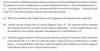
Let X be a random variable that represents the level of glucose in the blood (milligrams per deciliter of blood).
The distribution of X for a healthy person is normally distributed with men u = 85 and standard deviation o =
25. A person suffers from severe excess in insulin would have a lower level of glucose. A blood test with
result of X < 40 would be used as an indicator that medication is needed.
(a) What is the probability that a healthy person will be suggested with medication after a single test?
(b) A doctor uses the average result of 2 tests for diagnosis, that is X. The second test will be conducted
one week after the first test, so that the two test results are independent. For many healthy persons, each
has finished two tests, find the expectation and standard error of the distribution of X.
(c) The doctor suggests medication will be given only when the average level of glucoses in the 2 blood tests
is less than 40, that is X < 40, so to reduce the chance of unnecessary use of medication on a healthy
person. Use the distribution in part (b)) to find the probability that a healthy person will be suggested
with medication after 2 tests to verify this doctor's theory.
Transcribed Image Text:Let X be a random variable that represents the level of glucose in the blood (milligrams per deciliter of blood). The distribution of X for a healthy person is normally distributed with men u = 85 and standard deviation o = 25. A person suffers from severe excess in insulin would have a lower level of glucose. A blood test with result of X < 40 would be used as an indicator that medication is needed. (a) What is the probability that a healthy person will be suggested with medication after a single test? (b) A doctor uses the average result of 2 tests for diagnosis, that is X. The second test will be conducted one week after the first test, so that the two test results are independent. For many healthy persons, each has finished two tests, find the expectation and standard error of the distribution of X. (c) The doctor suggests medication will be given only when the average level of glucoses in the 2 blood tests is less than 40, that is X < 40, so to reduce the chance of unnecessary use of medication on a healthy person. Use the distribution in part (b)) to find the probability that a healthy person will be suggested with medication after 2 tests to verify this doctor's theory.
Solution
Bartleby Expert
SEE SOLUTION
Recommended textbooks for you
MATLAB: An Introduction with Applications
Statistics
ISBN:
9781119256830
Author:
Amos Gilat
Publisher:
John Wiley & Sons Inc
Probability and Statistics for Engineering and th…
Statistics
ISBN:
9781305251809
Author:
Jay L. Devore
Publisher:
Cengage Learning
Statistics for The Behavioral Sciences (MindTap C…
Statistics
ISBN:
9781305504912
Author:
Frederick J Gravetter, Larry B. Wallnau
Publisher:
Cengage Learning
Elementary Statistics: Picturing the World (7th E…
Statistics
ISBN:
9780134683416
Author:
Ron Larson, Betsy Farber
Publisher:
PEARSON
The Basic Practice of Statistics
Statistics
ISBN:
9781319042578
Author:
David S. Moore, William I. Notz, Michael A. Fligner
Publisher:
W. H. Freeman
Introduction to the Practice of Statistics
Statistics
ISBN:
9781319013387
Author:
David S. Moore, George P. McCabe, Bruce A. Craig
Publisher:
W. H. Freeman