Consider the case of a rotating wheel at rest and starting a clockwise rotation, meaning the negative direction of the angular velocity, and increasing (negatively) its value up to -12 rad/sec for 2 seconds. It then maintains a constant velocity for 2 seconds, and then uniformly reduces the magnitude of the velocity for 2 seconds until the wheel is momentarily stopped and restarts its rotation counter-clockwise with positive angular velocity, accelerating up to 20 rad/sec in 2 seconds and remaining at a constant rotation for 2 more seconds. Finally, the wheel stops gradually in 2 seconds. Next, you can see the graph of angular velocity versus time of this rotation: Apply the angular position equation. with θo=0, wo=0, substituting the value of the angular acceleration in the range from 0 to 2 seconds obtained in question 2, perform the tabulation of values to fill the following table; describe the type of parabola and draw the graph: Equation: θ=f(t) Concavity type: Vertex coordinates: Tabulation of values t θ 0 0.5 1 1.5 2 Graph Graph: θ vs t Continue applying the angular position equation, but now in the following form: Here you must substitute the values of initial angular velocity (ω1) and angular acceleration (α1), which correspond to the range from 2 to 4 seconds. Applying the value of t=2 seconds and the corresponding value θ from the table of question 17, obtain the value of θ1, in order to write the equation of the line, describe its characteristics, tabulate its values and draw the graphs: Equation: θ=f(t): Slope Tabulation of values t θ 2 2.5 3 3.5 4 Graph Graph: θ vs t Continue applying the angular position equation for the following range from 4 to 6 seconds: Here you must substitute the values of initial angular velocity (ω1) and angular acceleration (α1) which correspond to the range from 4 to 6 seconds. Applying the value of t=4 seconds and the corresponding value θ from the table of question 18, obtain the value of θ1, in order to write the equation of the line, describe its characteristics, tabulate its values and draw the graphs: Equation: θ=f(t) Type of concavity: Vertex coordinates: Tabulation of values t θ 4 4.5 5 5.5 6 Graph Graph: θ vs t Continue applying the angular position equation for the following range from 6 to 8 seconds: Here you must substitute the values of initial angular velocity (ω1) and angular acceleration (α1), which correspond to the range from 6 to 8 seconds. Applying the value of t=6 seconds and the corresponding value θ from the table of question 18, obtain the value of θ1, in order to write the equation of the line, describe its characteristics, tabulate its values and draw the graphs: Equation: θ=f(t) Type of concavity: Vertex coordinate: Tabulation of values t θ 6 6.5 7 7.5 8 Graph Graph: θ vs t Continue applying the angular position equation for the following range from 8 to 10 seconds: In which you must substitute the values of initial angular velocity (ω1) and angular acceleration (α1), which correspond to the range from 8 to 10 seconds. Applying the value of t=8 seconds and the corresponding value θ from the table of question 19, obtain the value of θ1, in order to write the equation of the line, describe its characteristics, tabulate its values and draw the graphs: Equation: θ=f(t): Slope Tabulation of values t θ 8 8.5 9 9.5 10 Graph Graph: θ vs t Continue applying the angular position equation for the following range from 10 to 12 seconds: Here you must substitute the values of initial angular velocity (ω1) and angular acceleration (α1), which correspond to the range from 10 to 12 seconds. Applying the value of t=10 seconds and the corresponding value θ from the table of question 20, obtain the value of θ1, in order to write the equation of the line, describe its characteristics, tabulate its values and draw the graphs: Equation: θ=f(t) Type of concavity: Vertex coordinates: Tabulation of values T θ 10 10.5 11 11.5 12 Finally, draw the full graph (range from 0 to 12 seconds) using the graphs drawn in the previous questions:


Angular Momentum
The momentum of an object is given by multiplying its mass and velocity. Momentum is a property of any object that moves with mass. The only difference between angular momentum and linear momentum is that angular momentum deals with moving or spinning objects. A moving particle's linear momentum can be thought of as a measure of its linear motion. The force is proportional to the rate of change of linear momentum. Angular momentum is always directly proportional to mass. In rotational motion, the concept of angular momentum is often used. Since it is a conserved quantity—the total angular momentum of a closed system remains constant—it is a significant quantity in physics. To understand the concept of angular momentum first we need to understand a rigid body and its movement, a position vector that is used to specify the position of particles in space. A rigid body possesses motion it may be linear or rotational. Rotational motion plays important role in angular momentum.
Moment of a Force
The idea of moments is an important concept in physics. It arises from the fact that distance often plays an important part in the interaction of, or in determining the impact of forces on bodies. Moments are often described by their order [first, second, or higher order] based on the power to which the distance has to be raised to understand the phenomenon. Of particular note are the second-order moment of mass (Moment of Inertia) and moments of force.
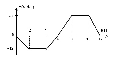
- Consider the case of a rotating wheel at rest and starting a clockwise rotation, meaning the negative direction of the
angular velocity , and increasing (negatively) its value up to -12 rad/sec for 2 seconds. It then maintains a constant velocity for 2 seconds, and then uniformly reduces the magnitude of the velocity for 2 seconds until the wheel is momentarily stopped and restarts its rotation counter-clockwise with positive angular velocity, accelerating up to 20 rad/sec in 2 seconds and remaining at a constant rotation for 2 more seconds. Finally, the wheel stops gradually in 2 seconds. Next, you can see the graph of angular velocity versus time of this rotation:
- Apply the angular position equation.
with θo=0, wo=0, substituting the value of the
|
Equation: |
|
|
Concavity type: |
|
|
Vertex coordinates: |
|
Tabulation of values
| t |
θ |
|
0 |
|
|
0.5 |
|
|
1 |
|
|
1.5 |
|
|
2 |
|
Graph
| Graph: θ vs t |
- Continue applying the angular position equation, but now in the following form:
Here you must substitute the values of initial angular velocity (ω1) and angular acceleration (α1), which correspond to the range from 2 to 4 seconds. Applying the value of t=2 seconds and the corresponding value θ from the table of question 17, obtain the value of θ1, in order to write the equation of the line, describe its characteristics, tabulate its values and draw the graphs:
|
Equation: |
|
|
Slope |
|
Tabulation of values
|
t |
θ |
|
2 |
|
|
2.5 |
|
|
3 |
|
|
3.5 |
|
|
4 |
|
Graph
|
Graph: θ vs t
|
- Continue applying the angular position equation for the following range from 4 to 6 seconds:
Here you must substitute the values of initial angular velocity (ω1) and angular acceleration (α1) which correspond to the range from 4 to 6 seconds. Applying the value of t=4 seconds and the corresponding value θ from the table of question 18, obtain the value of θ1, in order to write the equation of the line, describe its characteristics, tabulate its values and draw the graphs:
|
Equation: |
|
|
Type of concavity: |
|
|
Vertex coordinates: |
|
Tabulation of values
| t |
θ |
|
4 |
|
|
4.5 |
|
|
5 |
|
|
5.5 |
|
|
6 |
|
Graph
|
Graph: θ vs t
|
- Continue applying the angular position equation for the following range from 6 to 8 seconds:
Here you must substitute the values of initial angular velocity (ω1) and angular acceleration (α1), which correspond to the range from 6 to 8 seconds. Applying the value of t=6 seconds and the corresponding value θ from the table of question 18, obtain the value of θ1, in order to write the equation of the line, describe its characteristics, tabulate its values and draw the graphs:
|
Equation: |
|
|
Type of concavity: |
|
|
Vertex coordinate: |
|
Tabulation of values
| t |
θ |
|
6 |
|
|
6.5 |
|
|
7 |
|
|
7.5 |
|
|
8 |
|
Graph
|
Graph: θ vs t
|
- Continue applying the angular position equation for the following range from 8 to 10 seconds:
In which you must substitute the values of initial angular velocity (ω1) and angular acceleration (α1), which correspond to the range from 8 to 10 seconds. Applying the value of t=8 seconds and the corresponding value θ from the table of question 19, obtain the value of θ1, in order to write the equation of the line, describe its characteristics, tabulate its values and draw the graphs:
|
Equation: |
|
|
Slope |
|
Tabulation of values
| t |
θ |
|
8 |
|
|
8.5 |
|
|
9 |
|
|
9.5 |
|
|
10 |
|
Graph
|
Graph: θ vs t
|
- Continue applying the angular position equation for the following range from 10 to 12 seconds:
Here you must substitute the values of initial angular velocity (ω1) and angular acceleration (α1), which correspond to the range from 10 to 12 seconds. Applying the value of t=10 seconds and the corresponding value θ from the table of question 20, obtain the value of θ1, in order to write the equation of the line, describe its characteristics, tabulate its values and draw the graphs:
|
Equation: |
|
|
Type of concavity: |
|
|
Vertex coordinates: |
|
Tabulation of values
| T |
θ |
|
10 |
|
|
10.5 |
|
|
11 |
|
|
11.5 |
|
|
12 |
|
- Finally, draw the full graph (range from 0 to 12 seconds) using the graphs drawn in the previous questions:

Step by step
Solved in 3 steps with 1 images