(e) In previous problems, we assumed the x distribution was normal or approximately normal. Do we need to make such an assumption in this problem? Why or why not? Hint: Use the central limit theorem. O Yes. According to the central limit theorem, when n s 30, the x distribution is approximately normal. O No. According to the central limit theorem, when n 2 30, the x distribution is approximately normal. O No. According to the central limit theorem, when n s 30, the x distribution is approximately normal.
(e) In previous problems, we assumed the x distribution was normal or approximately normal. Do we need to make such an assumption in this problem? Why or why not? Hint: Use the central limit theorem. O Yes. According to the central limit theorem, when n s 30, the x distribution is approximately normal. O No. According to the central limit theorem, when n 2 30, the x distribution is approximately normal. O No. According to the central limit theorem, when n s 30, the x distribution is approximately normal.

MATLAB: An Introduction with Applications
6th Edition
ISBN:9781119256830
Author:Amos Gilat
Publisher:Amos Gilat
Chapter1: Starting With Matlab
Section: Chapter Questions
Problem 1P

Related questions
Topic Video
Question
100%
The home run percentage is the number of home runs per 100 times at bat. A random sample of 43 professional baseball players gave the following data for home run percentages.
1.6 2.4 1.2 6.6 2.3 0.0 1.8 2.5 6.5 1.8
2.7 2.0 1.9 1.3 2.7 1.7 1.3 2.1 2.8 1.4
3.8 2.1 3.4 1.3 1.5 2.9 2.6 0.0 4.1 2.9
1.9 2.4 0.0 1.8 3.1 3.8 3.2 1.6 4.2 0.0
1.2 1.8 2.4
I need help with part E
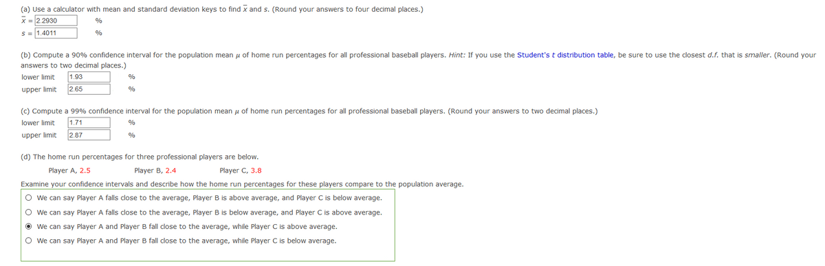
Transcribed Image Text:(a) Use a calculator with mean and standard deviation keys to find x and s. (Round your answers to four decimal places.)
x =2.2930
%
S = 1.4011
%
(b) Compute a 90% confidence interval for the population mean u of home run percentages for all professional baseball players. Hint: If you use the Student's t distribution table, be sure to use the closest d.f. that is smaller. (Round your
answers to two decimal places.)
lower limit
1.93
%
upper limit
2.65
%
(c) Compute a 99% confidence interval for the population mean u of home run percentages for all professional baseball players. (Round your answers to two decimal places.)
lower limit
1.71
%
upper limit
2.87
%
(d) The home run percentages for three professional players are below.
Player A, 2.5
Player B, 2.4
Player C, 3.8
Examine your confidence intervals and describe how the home run percentages for these players compare to the population average.
O we can say Player A falls close to the average, Player B is above average, and Player C is below average.
O we can say Player A falls close to the average, Player B is below average, and Player C is above average.
O We can say Player A and Player B fall close to the average, while Player C is above average.
O we can say Player A and Player B fall close to the average, while Player C is below average.
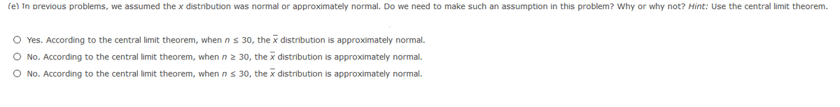
Transcribed Image Text:(e) In previous problems, we assumed the x distribution was normal or approximately normal. Do we need to make such an assumption in this problem? Why or why not? Hint: Use the central limit theorem.
O Yes. According to the central limit theorem, when n < 30, the x distribution is approximately normal.
O No. According to the central limit theorem, when n 2 30, the x distribution is approximately normal.
O No. According to the central limit theorem, when n < 30, the x distribution is approximately normal.
Expert Solution
This question has been solved!
Explore an expertly crafted, step-by-step solution for a thorough understanding of key concepts.

This is a popular solution!

Trending now
This is a popular solution!

Step by step
Solved in 2 steps

Knowledge Booster


Learn more about
Need a deep-dive on the concept behind this application? Look no further. Learn more about this topic, statistics and related others by exploring similar questions and additional content below.Recommended textbooks for you
MATLAB: An Introduction with Applications
Statistics
ISBN:
9781119256830
Author:
Amos Gilat
Publisher:
John Wiley & Sons Inc

Probability and Statistics for Engineering and th…
Statistics
ISBN:
9781305251809
Author:
Jay L. Devore
Publisher:
Cengage Learning

Statistics for The Behavioral Sciences (MindTap C…
Statistics
ISBN:
9781305504912
Author:
Frederick J Gravetter, Larry B. Wallnau
Publisher:
Cengage Learning
MATLAB: An Introduction with Applications
Statistics
ISBN:
9781119256830
Author:
Amos Gilat
Publisher:
John Wiley & Sons Inc
Probability and Statistics for Engineering and th…
Statistics
ISBN:
9781305251809
Author:
Jay L. Devore
Publisher:
Cengage Learning
Statistics for The Behavioral Sciences (MindTap C…
Statistics
ISBN:
9781305504912
Author:
Frederick J Gravetter, Larry B. Wallnau
Publisher:
Cengage Learning

Elementary Statistics: Picturing the World (7th E…
Statistics
ISBN:
9780134683416
Author:
Ron Larson, Betsy Farber
Publisher:
PEARSON

The Basic Practice of Statistics
Statistics
ISBN:
9781319042578
Author:
David S. Moore, William I. Notz, Michael A. Fligner
Publisher:
W. H. Freeman

Introduction to the Practice of Statistics
Statistics
ISBN:
9781319013387
Author:
David S. Moore, George P. McCabe, Bruce A. Craig
Publisher:
W. H. Freeman