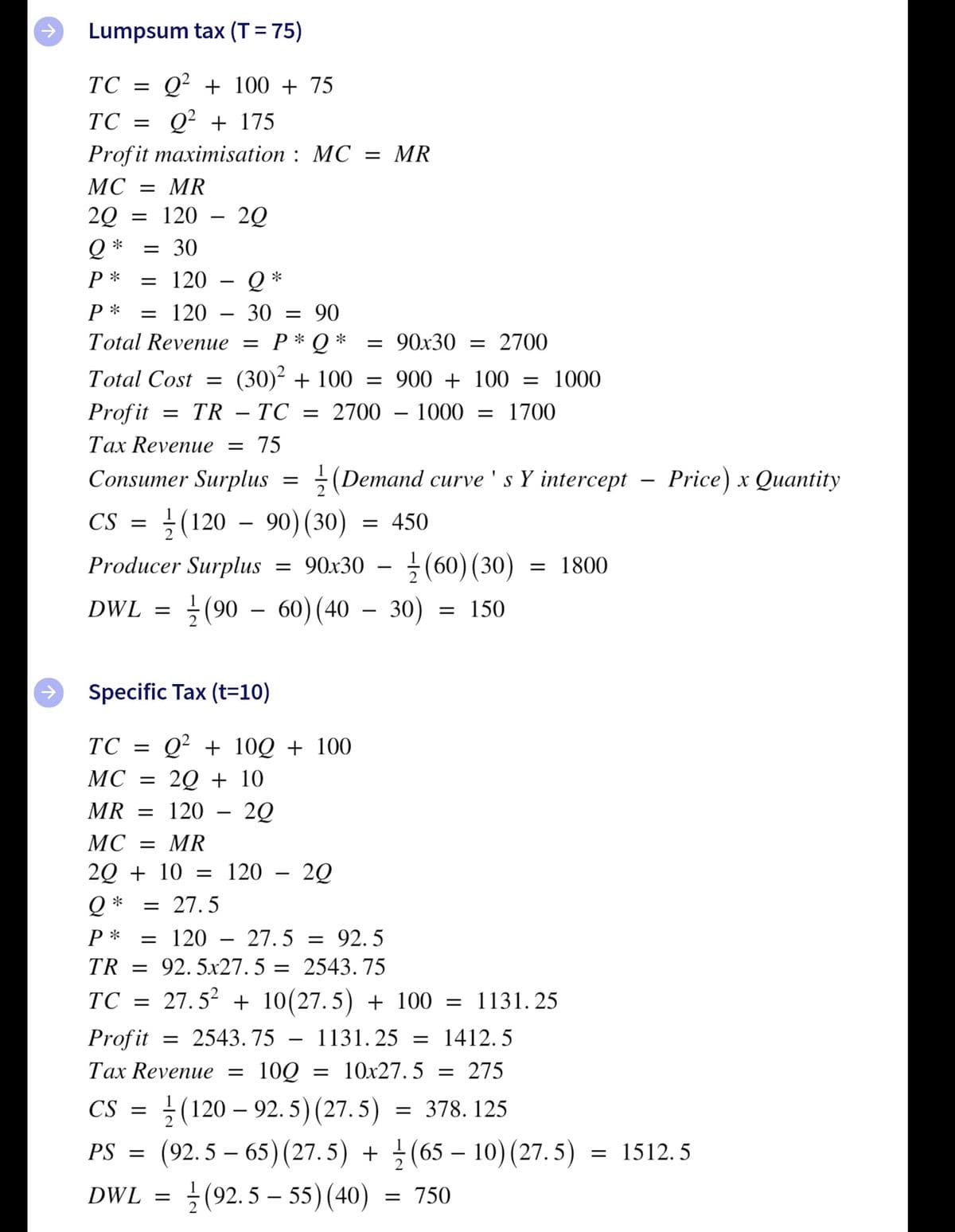
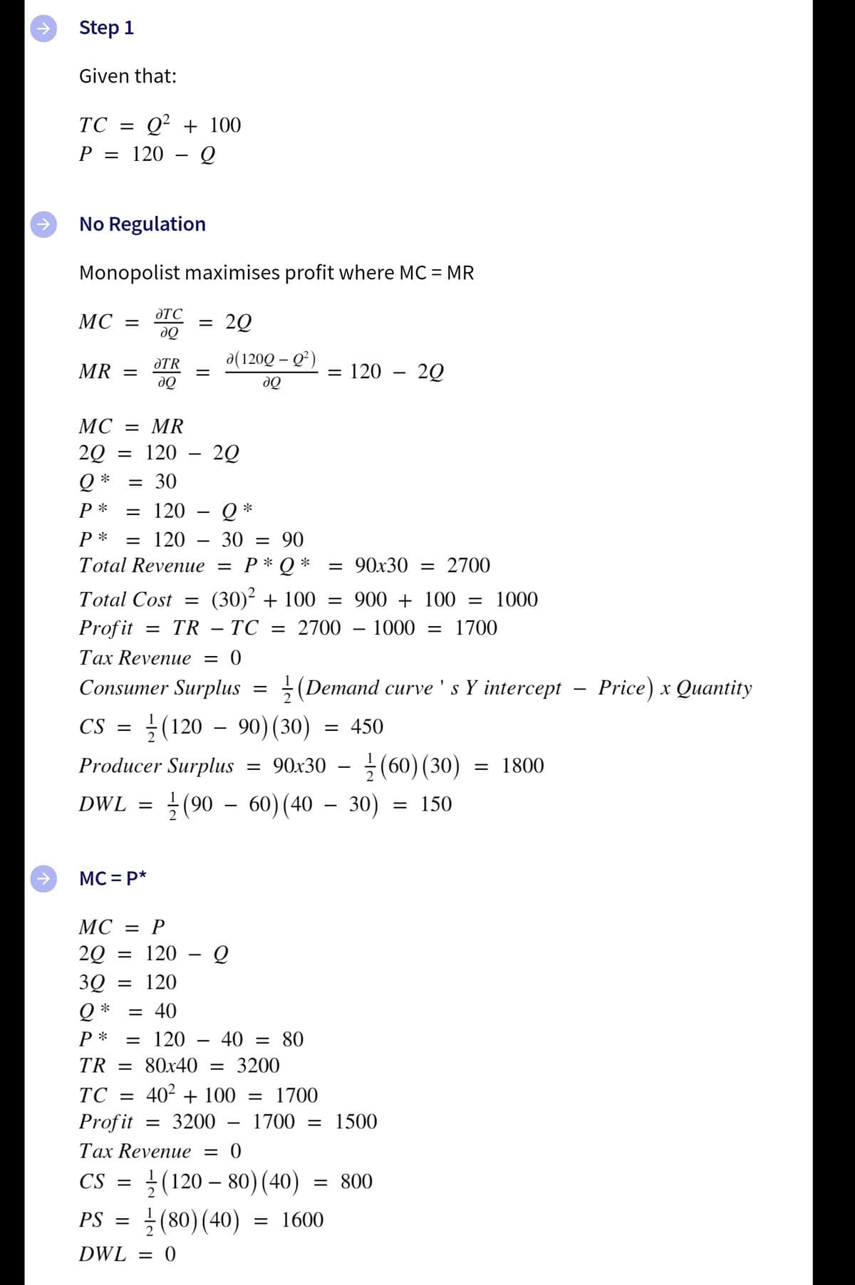
Fill-up the following table relating to monopoly operations and regulations given the following total cost and inverse demand functions: No Regulation MC-Pricing (MC = P*) w/ Lump Sum Tax (T = 75) w/ Specific Tax (t = 10) Profit Equation Q* P* TR at Q* TC at Q* Profit at Q* Tax Revenue Consumer Surplus Producer Surplus Deadweight Loss 2.) Choose one type of regulation you analyzed in number 1 and graphically illustrate the results.


Hello my dear tutor!
I just want to ask for help whether the answers in the given pictures are correct. If it's not, please help me recheck and resolve it. Please refer to the given pictures below for the answers.
After verifying the given answers shown in the subsequent picture. PLEASE TALLY AND FILL UP AND PROVIDE THE NECESSARY INFORMATION FROM THE TABLE BELOW. Answer also number 2.
NOTE: Type only your answers. Please do not handwritten your answers.
1.) Fill-up the following table relating to
|
|
No Regulation |
MC-Pricing (MC = P*) |
w/ Lump Sum Tax (T = 75) |
w/ Specific Tax (t = 10) |
|
Profit Equation |
|
|
|
|
|
Q* |
|
|
|
|
|
P* |
|
|
|
|
|
TR at Q* |
|
|
|
|
|
TC at Q* |
|
|
|
|
|
Profit at Q* |
|
|
|
|
|
Tax Revenue |
|
|
|
|
|
|
|
|
|
|
|
|
|
|
|
|
|
|
|
|
|
|
2.) Choose one type of regulation you analyzed in number 1 and graphically illustrate the results.
NOTE: Type only your answers. Please do not handwritten your answers.


Trending now
This is a popular solution!

Step by step
Solved in 2 steps with 3 images


