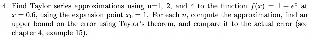
Find Taylor series approximations using n=1, 2, and 4 to the function f(x) = 1 + eª at x = 0.6, using the expansion point x = 1. For each n, compute the approximation, find an upper bound on the error using Taylor's theorem, and compare it to the actual error (see chapter 4, example 15).
Find Taylor series approximations using n=1, 2, and 4 to the function f(x) = 1 + eª at x = 0.6, using the expansion point x = 1. For each n, compute the approximation, find an upper bound on the error using Taylor's theorem, and compare it to the actual error (see chapter 4, example 15).

Advanced Engineering Mathematics
10th Edition
ISBN:9780470458365
Author:Erwin Kreyszig
Publisher:Erwin Kreyszig
Chapter2: Second-order Linear Odes
Section: Chapter Questions
Problem 1RQ

Related questions
Question
Transcribed Image Text:4. Find Taylor series approximations using n=1, 2, and 4 to the function f(x) = 1 + eª at
X = 0.6, using the expansion point xo 1. For each n, compute the approximation, find an
upper bound on the error using Taylor's theorem, and compare it to the actual error (see
chapter 4, example 15).
=
![Example 16. Use Taylor's theorem with n = 2 to approximate sin(x) at x = 1.1, using
the expansion point xo = 1. Find a bound on the error using Taylor's theorem and com-
pare the bound to the actual error.
First, we calculate:
f(1) = sin(1),
f'(1) = cos(1), f" (1) =
sin(1).
Thus we can approximate f by: f(x) = sin(1) + cos(1)(x − 1) – sin(1)(x - 1)² with error
term cos(c)(x - 1)³, where c is not known precisely, but is known to live in the interval
[1, 1.1]. Hence at x = 1.1, we get the approximation
f(1.1)
sin(1) + (0.1) cos(1) - (0.01)-
The error term was given by - cos(c)(x - 1)³, with c unknown but in the interval [1, 1.1].
We know that | cos(x)| ≤ 1, so we can upper bound the error by
cos(c)
6
error:
(1.11)
1-1)³| ≤ (0.001):
sin(1)
2
Using MATLAB, we calculate this approximation, the actual answer, and the actual
| co
cos(c)
6
This is now quite close to the actual error.
(0.001) 1.6667e - 4.
(1.1-1)³| ≤ 3
<
=
=
>> approx-sin (1) + (0.1) *cos (1)-0.01/2*sin (1);
>> exact=sin (1.1);
.55
>> error approx-exact;
>> disp([approx, exact, error]);
0.891293860470671 0.891207360061435 0.000086500409236
0.891293860470671.
Note the actual error was smaller than the estimated error, but the estimated er-
ror was a guarantee of what the maximum error can be. Note that cos(1.1) ≈ 0.45 ≤
cos(c) ≤ 0.55= cos(1), so we can improve the error bound by using | cos(c)| ≤ 0.55,
which gives the improved upper bound on the error estimate:
6
-(0.001) 9.1667e - 5.
=](/v2/_next/image?url=https%3A%2F%2Fcontent.bartleby.com%2Fqna-images%2Fquestion%2F0a5ac3c6-e4ab-423a-91e1-ff33bdae0d07%2F26b167fd-5d8b-4d8c-aff0-1a0d5d5fc842%2Fz8ibgd4f_processed.png&w=3840&q=75)
Transcribed Image Text:Example 16. Use Taylor's theorem with n = 2 to approximate sin(x) at x = 1.1, using
the expansion point xo = 1. Find a bound on the error using Taylor's theorem and com-
pare the bound to the actual error.
First, we calculate:
f(1) = sin(1),
f'(1) = cos(1), f" (1) =
sin(1).
Thus we can approximate f by: f(x) = sin(1) + cos(1)(x − 1) – sin(1)(x - 1)² with error
term cos(c)(x - 1)³, where c is not known precisely, but is known to live in the interval
[1, 1.1]. Hence at x = 1.1, we get the approximation
f(1.1)
sin(1) + (0.1) cos(1) - (0.01)-
The error term was given by - cos(c)(x - 1)³, with c unknown but in the interval [1, 1.1].
We know that | cos(x)| ≤ 1, so we can upper bound the error by
cos(c)
6
error:
(1.11)
1-1)³| ≤ (0.001):
sin(1)
2
Using MATLAB, we calculate this approximation, the actual answer, and the actual
| co
cos(c)
6
This is now quite close to the actual error.
(0.001) 1.6667e - 4.
(1.1-1)³| ≤ 3
<
=
=
>> approx-sin (1) + (0.1) *cos (1)-0.01/2*sin (1);
>> exact=sin (1.1);
.55
>> error approx-exact;
>> disp([approx, exact, error]);
0.891293860470671 0.891207360061435 0.000086500409236
0.891293860470671.
Note the actual error was smaller than the estimated error, but the estimated er-
ror was a guarantee of what the maximum error can be. Note that cos(1.1) ≈ 0.45 ≤
cos(c) ≤ 0.55= cos(1), so we can improve the error bound by using | cos(c)| ≤ 0.55,
which gives the improved upper bound on the error estimate:
6
-(0.001) 9.1667e - 5.
=
Expert Solution
This question has been solved!
Explore an expertly crafted, step-by-step solution for a thorough understanding of key concepts.

This is a popular solution!

Trending now
This is a popular solution!

Step by step
Solved in 2 steps with 2 images

Recommended textbooks for you
Advanced Engineering Mathematics
Advanced Math
ISBN:
9780470458365
Author:
Erwin Kreyszig
Publisher:
Wiley, John & Sons, Incorporated

Numerical Methods for Engineers
Advanced Math
ISBN:
9780073397924
Author:
Steven C. Chapra Dr., Raymond P. Canale
Publisher:
McGraw-Hill Education

Introductory Mathematics for Engineering Applicat…
Advanced Math
ISBN:
9781118141809
Author:
Nathan Klingbeil
Publisher:
WILEY
Advanced Engineering Mathematics
Advanced Math
ISBN:
9780470458365
Author:
Erwin Kreyszig
Publisher:
Wiley, John & Sons, Incorporated
Numerical Methods for Engineers
Advanced Math
ISBN:
9780073397924
Author:
Steven C. Chapra Dr., Raymond P. Canale
Publisher:
McGraw-Hill Education
Introductory Mathematics for Engineering Applicat…
Advanced Math
ISBN:
9781118141809
Author:
Nathan Klingbeil
Publisher:
WILEY

Mathematics For Machine Technology
Advanced Math
ISBN:
9781337798310
Author:
Peterson, John.
Publisher:
Cengage Learning,

