I want to know how to get plots like in the image in MATLAB. I have the following code. With the angular velocity data, how do I get a figure like show in the image I = [0.3; 0.2; 0.4]; w_per1 = [0.1; 0.001; 0.001]; w_per2 = [0.001; 0.1; 0.001]; w_per3 = [0.001; 0.001; 0.1]; L = [0;0;0]; t = 0:300; sigma = [0.3; 0.3; 0.3]; % Finidng EP from MRP EP = MRPtoEP(sigma) % Using ode45 to integrate KDE options = odeset('RelTol',1e-10,'AbsTol',1e-10); [t, y] = ode45(@dwdt_KDE_EP, t, [EP; w_per2], options); % Extract the Euler parameters and angular velocities w_p1 = y(:, 5:7)'; function dqwdt = dwdt_KDE_EP(~,EPw) I = [0.3; 0.2; 0.4]; L = [0;0;0]; EP = EPw(1:4); w = EPw(5:7); dqdt = zeros(4,1); dwdt = zeros(3,1); dqdt(1) = 0.5*(EP(4)*w(1) - EP(3)*w(2) + EP(2)*w(3)); dqdt(2) = 0.5*(EP(3)*w(1) + EP(4)*w(2) - EP(1)*w(3)); dqdt(3) = 0.5*(-EP(2)*w(1) + EP(1)*w(2) + EP(4)*w(3)); dqdt(4) = -0.5*(EP(1)*w(1) + EP(2)*w(2) + EP(3)*w(3)); dwdt(1) = (-(I(3) - I(2))*w(2)*w(3) + L(1)) / I(1); dwdt(2) = (-(I(1) - I(3))*w(3)*w(1) + L(2)) / I(2); dwdt(3) = (-(I(2) - I(1))*w(1)*w(2) + L(3)) / I(3); % Combine the time derivatives into a single vector dqwdt = [dqdt; dwdt]; end function [EP] = MRPtoEP(sigma) EP1 = (2*sigma(1)) / (1 + dot(sigma, sigma)); EP2 = (2*sigma(2)) / (1 + dot(sigma, sigma)); EP3 = (2*sigma(3)) / (1 + dot(sigma, sigma)); EP4 = (1 - dot(sigma, sigma)) / (1 + dot(sigma, sigma)); EP = [EP1; EP2; EP3; EP4]; end


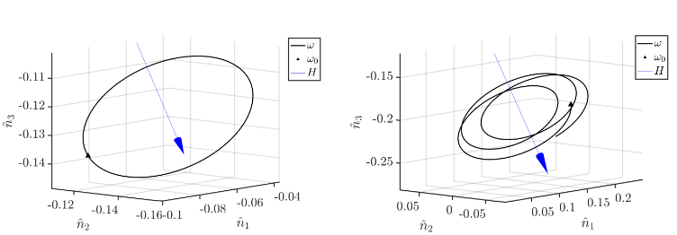
I want to know how to get plots like in the image in MATLAB. I have the following code. With the angular velocity data, how do I get a figure like show in the image
I = [0.3; 0.2; 0.4];
w_per1 = [0.1; 0.001; 0.001];
w_per2 = [0.001; 0.1; 0.001];
w_per3 = [0.001; 0.001; 0.1];
L = [0;0;0];
t = 0:300;
sigma = [0.3; 0.3; 0.3];
% Finidng EP from MRP
EP = MRPtoEP(sigma)
% Using ode45 to integrate KDE
options = odeset('RelTol',1e-10,'AbsTol',1e-10);
[t, y] = ode45(@dwdt_KDE_EP, t, [EP; w_per2], options);
% Extract the Euler parameters and angular velocities
w_p1 = y(:, 5:7)';
function dqwdt = dwdt_KDE_EP(~,EPw)
I = [0.3; 0.2; 0.4];
L = [0;0;0];
EP = EPw(1:4);
w = EPw(5:7);
dqdt = zeros(4,1);
dwdt = zeros(3,1);
dqdt(1) = 0.5*(EP(4)*w(1) - EP(3)*w(2) + EP(2)*w(3));
dqdt(2) = 0.5*(EP(3)*w(1) + EP(4)*w(2) - EP(1)*w(3));
dqdt(3) = 0.5*(-EP(2)*w(1) + EP(1)*w(2) + EP(4)*w(3));
dqdt(4) = -0.5*(EP(1)*w(1) + EP(2)*w(2) + EP(3)*w(3));
dwdt(1) = (-(I(3) - I(2))*w(2)*w(3) + L(1)) / I(1);
dwdt(2) = (-(I(1) - I(3))*w(3)*w(1) + L(2)) / I(2);
dwdt(3) = (-(I(2) - I(1))*w(1)*w(2) + L(3)) / I(3);
% Combine the time derivatives into a single
dqwdt = [dqdt; dwdt];
end
function [EP] = MRPtoEP(sigma)
EP1 = (2*sigma(1)) / (1 + dot(sigma, sigma));
EP2 = (2*sigma(2)) / (1 + dot(sigma, sigma));
EP3 = (2*sigma(3)) / (1 + dot(sigma, sigma));
EP4 = (1 - dot(sigma, sigma)) / (1 + dot(sigma, sigma));
EP = [EP1; EP2; EP3; EP4];
end

Step by step
Solved in 3 steps with 4 images


