In ongoing economic analyses, the U.S. federal government compares per capita incomes not only among different states but also for the same state at different times. For the 50 states, the least-squares regression equation relating the 1980 per capita income and the 1999 per capita income is y =7.97+1.97x, with x denoting 1980 per capita income and y denoting 1999 per capita income. The standard error of the slope of this least-squares regression line is approximately 1.65. (Source: U.S. Bureau of Economic Analysis, Survey of Current Business, May 2000). Based on this information, test for a significant linear relationship between the variables x and y by doing a hypothesis test regarding the population slope B,. (Assume that the variable y follows a normal distribution for each value of x and that the other regression assumptions are satisfied.) Use the 0.10 level of significance, and perform a two-tailed test. Then complete the parts below. (If necessary, consult a list of formulas.) (a) State the null hypothesis H and the alternative hypothesis H,. B H, :0 H :0 O=0 OSO (b) Determine the type of test statistic to use. O
In ongoing economic analyses, the U.S. federal government compares per capita incomes not only among different states but also for the same state at different times. For the 50 states, the least-squares regression equation relating the 1980 per capita income and the 1999 per capita income is y =7.97+1.97x, with x denoting 1980 per capita income and y denoting 1999 per capita income. The standard error of the slope of this least-squares regression line is approximately 1.65. (Source: U.S. Bureau of Economic Analysis, Survey of Current Business, May 2000). Based on this information, test for a significant linear relationship between the variables x and y by doing a hypothesis test regarding the population slope B,. (Assume that the variable y follows a normal distribution for each value of x and that the other regression assumptions are satisfied.) Use the 0.10 level of significance, and perform a two-tailed test. Then complete the parts below. (If necessary, consult a list of formulas.) (a) State the null hypothesis H and the alternative hypothesis H,. B H, :0 H :0 O=0 OSO (b) Determine the type of test statistic to use. O

College Algebra
7th Edition
ISBN:9781305115545
Author:James Stewart, Lothar Redlin, Saleem Watson
Publisher:James Stewart, Lothar Redlin, Saleem Watson
Chapter1: Equations And Graphs
Section: Chapter Questions
Problem 10T: Olympic Pole Vault The graph in Figure 7 indicates that in recent years the winning Olympic men’s...

Related questions
Question
Question #17
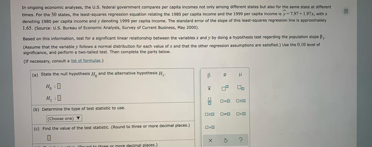
Transcribed Image Text:In ongoing economic analyses, the U.S. federal government compares per capita incomes not only among different states but also for the same state at different
times. For the 50 states, the least-squares regression equation relating the 1980 per capita income and the 1999 per capita income is y =7.97+1.97x, with x
denoting 1980 per capita income and y denoting 1999 per capita income. The standard error of the slope of this least-squares regression line is approximately
1.65. (Source: U.S. Bureau of Economic Analysis, Survey of Current Business, May 2000).
Based on this information, test for a significant linear relationship between the variables
and y by doing a hypothesis test regarding the population slope ß -
(Assume that the variable y follows a normal distribution for each value of x and that the other regression assumptions are satisfied.) Use the 0.10 level of
significance, and perform a two-tailed test. Then complete the parts below.
(If necessary, consult a list of formulas.)
(a) State the null hypothesis H, and the alternative hypothesis H,.
H :0
H, :0
D=0
OSO
(b) Determine the type of test statistic to use.
(Choose one) ▼
(c) Find the value of the test statistic. (Round to three or more decimal places.)
(Dound to three or more decimal places.)
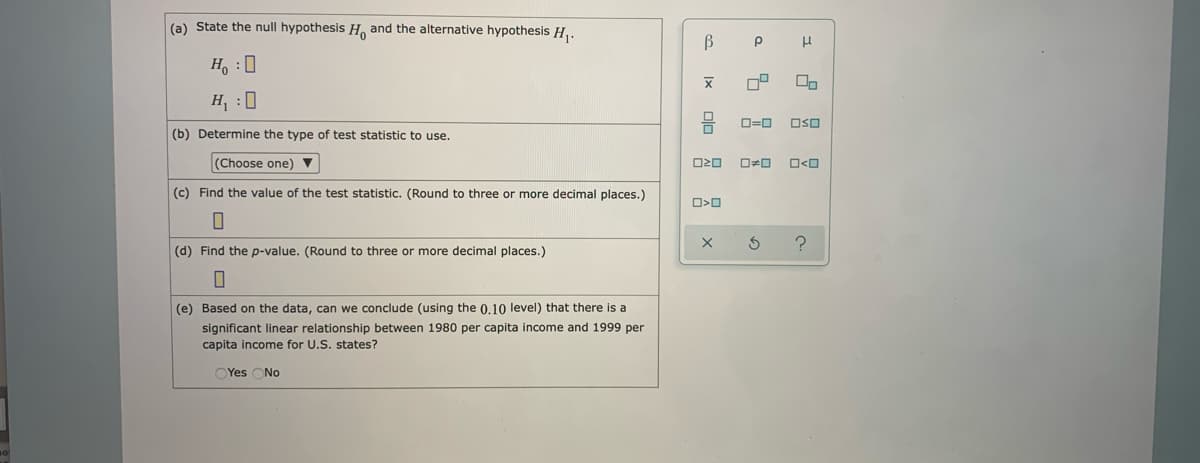
Transcribed Image Text:(a) State the null hypothesis H and the alternative hypothesis H,.
B
H, :0
H :0
O=0
OSO
(b) Determine the type of test statistic to use.
(Choose one) ▼
ロロ
O<O
(c) Find the value of the test statistic. (Round to three or more decimal places.)
(d) Find the p-value. (Round to three or more decimal places.)
(e) Based on the data, can we conclude (using the 0,10 level) that there is a
significant linear relationship between 1980 per capita income and 1999 per
capita income for U.S. states?
OYes ONo
olo 2
Expert Solution
This question has been solved!
Explore an expertly crafted, step-by-step solution for a thorough understanding of key concepts.

This is a popular solution!

Trending now
This is a popular solution!

Step by step
Solved in 2 steps with 2 images

Recommended textbooks for you
College Algebra
Algebra
ISBN:
9781305115545
Author:
James Stewart, Lothar Redlin, Saleem Watson
Publisher:
Cengage Learning

Linear Algebra: A Modern Introduction
Algebra
ISBN:
9781285463247
Author:
David Poole
Publisher:
Cengage Learning
College Algebra
Algebra
ISBN:
9781305115545
Author:
James Stewart, Lothar Redlin, Saleem Watson
Publisher:
Cengage Learning
Linear Algebra: A Modern Introduction
Algebra
ISBN:
9781285463247
Author:
David Poole
Publisher:
Cengage Learning