Investigation Results – Using the given data, investigate the possible relationships between Life Expectancy as the response variable (y) and each of the three explanatory variables (x). For each x variable, you will complete the following steps. Construct a scatter diagram displaying the relationship between x and y. You can use graph paper and draw the diagram by hand, use your calculator and take a picture of the screen, or use the online site: https://www.desmos.com/, whi


*** Answer 1-3 please ***
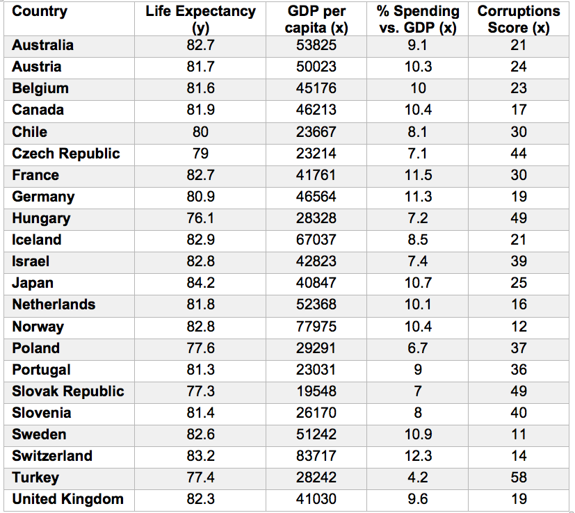
Investigation Results – Using the given data, investigate the possible relationships between Life Expectancy as the response variable (y) and each of the three explanatory variables (x). For each x variable, you will complete the following steps.
Construct a
You can use graph paper and draw the diagram by hand, use your calculator and take a picture of the screen, or use the online site: https://www.desmos.com/, which will allow you to print or save your diagram.
Calculate and state the sample
Describe the type of correlation, if any, and interpret the correlation in the context o-f the data.
Determine if the correlation is significant. Use α = 0.05 and show all steps of this process.
Inferences - Write at least one paragraph for each of the following questions. In the paragraph, you should explain as though you are talking to someone that is not in a statistics class. In other words, give details.
Now that you have investigated the relationships between y and each of the three different x variables, which explanatory variable (x) is the best predictor for Life Expectancy (y)? To defend your choice, discuss your investigation results for each
(x, y) pairing from part 1, including correlation coefficients and their significance.
Calculate the regression equation for the relationship you determined to be the “best” in part a. What is the “rate of change” of your equation? Using this rate of change, describe the behavior of Life Expectancy (y) as a result of changes in the explanatory variable (x) that you chose.
- Discuss the overall fitness of your regression line to the data set, by graphing the line on your scatter plot and by considering the correlation coefficient. Would you say that the explanatory variable you chose is reasonably predictive of Life Expectancy? Why or why not?
2. You may have noticed that the United States was not included in the data set you were given. Below are the relevant statistics for the United States.
|
United States |
|
|
Life Expectancy (y) |
78.5 |
|
|
|
|
GDP per capita (x) |
59531.7 |
|
% Spending versus GDP (x) |
17.17 |
|
Inverted Corruptions Score (x) |
24 |
Using the regression model that you calculated in part b, plug in the appropriate x-value for the United States to make a prediction of Life Expectancy. Also, calculate the residual value (difference between your prediction and the actual value). Does the United States seem to fit in your model or is it an outlier? Give the reason(s) for your answer.
3. Summarize your findings. If you were part of a United Nations team tasked with researching and making recommendations to member countries to improve life expectancy for their citizens, what would be your next steps?


Trending now
This is a popular solution!

Step by step
Solved in 3 steps with 3 images


