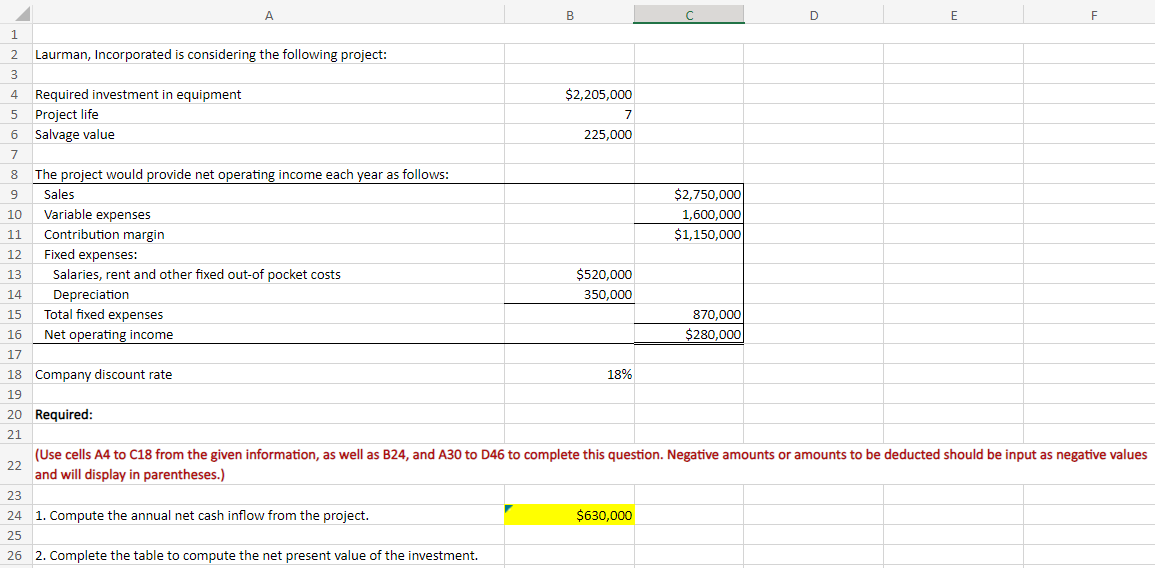
Laurman, Incorporated is considering the following project: Required investment in equipment Project life Salvage value The project would provide net operating income each year as follows: Sales Variable expenses Contribution margin Fixed expenses: Salaries, rent and other fixed out-of pocket costs Depreciation Total fixed expenses Net operating income Company discount rate Required: 1. Compute the annual net cash inflow from the project. $2,205,000 2. Complete the table to compute the net present value of the investment. 7 225,000 $520,000 350,000 18% (Use cells A4 to C18 from the given information, as well as B24, and A30 to D46 to complete this question. Negative amounts or amounts to and will display in parentheses.) $2,750,000 1,600,000 $1,150,000 $630,000 870,000 $280,000
Laurman, Incorporated is considering the following project: Required investment in equipment Project life Salvage value The project would provide net operating income each year as follows: Sales Variable expenses Contribution margin Fixed expenses: Salaries, rent and other fixed out-of pocket costs Depreciation Total fixed expenses Net operating income Company discount rate Required: 1. Compute the annual net cash inflow from the project. $2,205,000 2. Complete the table to compute the net present value of the investment. 7 225,000 $520,000 350,000 18% (Use cells A4 to C18 from the given information, as well as B24, and A30 to D46 to complete this question. Negative amounts or amounts to and will display in parentheses.) $2,750,000 1,600,000 $1,150,000 $630,000 870,000 $280,000

Essentials Of Investments
11th Edition
ISBN:9781260013924
Author:Bodie, Zvi, Kane, Alex, MARCUS, Alan J.
Publisher:Bodie, Zvi, Kane, Alex, MARCUS, Alan J.
Chapter1: Investments: Background And Issues
Section: Chapter Questions
Problem 1PS

Related questions
Question
I need help with the attached empty fields
Laurman, Incorporated is considering a new project and has provided the details of the project. The Controller has asked you to compute various capital budgeting methods to help aid in the decision to pursue the investment.
- Cell Reference: Allows you to refer to data from another cell in the worksheet. If you entered “=B5” into a blank cell, the formula would output the value from cell B5.
- Basic Math Functions: Allow you to use the basic math symbols to perform mathematical functions. You can use the following keys: + (plus sign to add), - (minus sign to subtract), * (asterisk sign to multiply), and / (forward slash to divide). For example, if you entered “=B4+B5” in a blank cell, the formula would add the values from those cells and output the result.
- SUM Function: Allows you to refer to multiple cells and adds all the values. You can add individual cell references or ranges. If you entered “=SUM(C4,C5,C6)” into a blank cell, the formula would output the result of adding those three separate cells. Similarly, if you entered “=SUM(C4:C6)”, the formula would output the same result of adding those cells.
- RATE Function: Allows you to return the interest rate per period. The syntax of the RATE function is “=RATE(nper,pmt,pv,[fv],[type],[guess])” the result is the percentage interest rate value for the related inputs. The nper argument is the total number of payment periods. The pmt argument is the payment made each period that does not change over the life of the investment and this argument must be included if the [fv] argument is not included. The pv argument is the present value, or the total amount that series of future payments is worth now. The [fv] argument is the
future value , or the cash basis to attain after the last payment is made and this argument must be included if the pmt argument is omitted. The [type] argument is a logical value of 0 or 1, which indicates when the payments are due where 1 is the payment at the beginning of the period and 0, is the payment at the end of the period. Both the [fv] and [type] values are optional arguments to have the formula work, which is why they are surrounded by brackets in the syntax, however, these values would not be entered with brackets in the actual function. The [guess] argument is also optional and is your guess for what the rate will be, however, if omitted the system assumes a guess of 10 percent. For this assignment, please include both the [pmt] and [fv] arguments, but leave out the [type] and [guess] arguments from the function. Also, the pv argument should be entered as negative value. - PV Function: Allows you to perform a present-value calculation.The syntax of the PV function is “=PV(rate,nper,pmt,[fv],[type])” and its output is the total amount that a series of future payments is worth now (also known as the present value). The rate argument is the interest rate per period. The nper argument is the total number of payment periods. The pmt argument is the payment made each period that does not change over the life of the investment, and this argument must be included if the [fv] argument is not included. The [fv] argument is the future value, or the cash basis to attain after the last payment is made; this argument must be included if the pmt argument is omitted. The [type] argument is a logical value of 0 or 1, which indicates when the payments are due, where 1 is the payment at the beginning of the period and 0 is the payment at the end of the period. Both the [fv] and [type] values are optional arguments to include, which is why they are surrounded by brackets in the syntax. However, these values would not be entered with brackets in the actual function
Transcribed Image Text:1
2
3
4 Required investment in equipment
5 Project life
6 Salvage value
7
8 The project would provide net operating income each year as follows:
9
Sales
10
Variable expenses
11 Contribution margin
12
13
Laurman, Incorporated is considering the following project:
14
15
16
17
18 Company discount rate
19
22
A
Fixed expenses:
Salaries, rent and other fixed out-of pocket costs
Depreciation
Total fixed expenses
Net operating income
20 Required:
21
B
23
24 1. Compute the annual net cash inflow from the project.
25
26 2. Complete the table to compute the net present value of the investment.
$2,205,000
7
225,000
$520,000
350,000
18%
с
$630,000
$2,750,000
1,600,000
$1,150,000
870,000
$280,000
D
E
(Use cells A4 to C18 from the given information, as well as B24, and A30 to D46 to complete this question. Negative amounts or amounts to be deducted should be input as negative values
and will display in parentheses.)
F
Transcribed Image Text:A
25
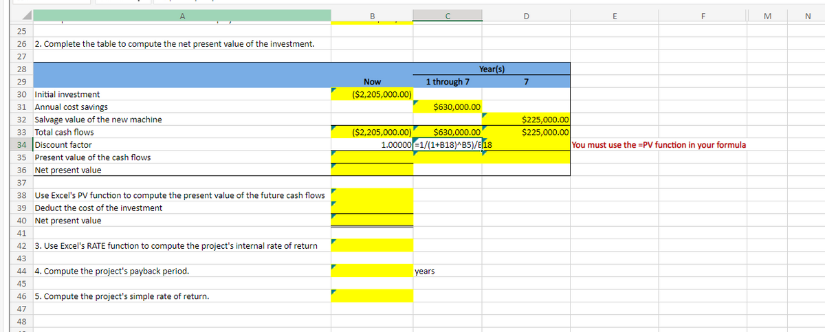
26 2. Complete the table to compute the net present value of the investment.
27
28
29
30 Initial investment
31 Annual cost savings
32 Salvage value of the new machine
33 Total cash flows
34 Discount factor
35 Present value of the cash flows
36 Net present value
37
38
Use Excel's PV function to compute the present value of the future cash flows
39 Deduct the cost of the investment
40 Net present value
41
42
3. Use Excel's RATE function to compute the project's internal rate of return
43
44
45
4. Compute the project's payback period.
46 5. Compute the project's simple rate of return.
47
48
B
Now
($2,205,000.00)
1 through 7
Year(s)
$630,000.00
($2,205,000.00) $630,000.00
1.00000=1/(1+B18)^B5)/E 18
years
D
7
$225,000.00
$225,000.00
E
F
You must use the =PV function in your formula
M
N
Expert Solution
This question has been solved!
Explore an expertly crafted, step-by-step solution for a thorough understanding of key concepts.

This is a popular solution!

Trending now
This is a popular solution!

Step by step
Solved in 3 steps with 3 images

Knowledge Booster


Learn more about
Need a deep-dive on the concept behind this application? Look no further. Learn more about this topic, finance and related others by exploring similar questions and additional content below.Recommended textbooks for you
Essentials Of Investments
Finance
ISBN:
9781260013924
Author:
Bodie, Zvi, Kane, Alex, MARCUS, Alan J.
Publisher:
Mcgraw-hill Education,

Essentials Of Investments
Finance
ISBN:
9781260013924
Author:
Bodie, Zvi, Kane, Alex, MARCUS, Alan J.
Publisher:
Mcgraw-hill Education,
Foundations Of Finance
Finance
ISBN:
9780134897264
Author:
KEOWN, Arthur J., Martin, John D., PETTY, J. William
Publisher:
Pearson,
Fundamentals of Financial Management (MindTap Cou…
Finance
ISBN:
9781337395250
Author:
Eugene F. Brigham, Joel F. Houston
Publisher:
Cengage Learning
Corporate Finance (The Mcgraw-hill/Irwin Series i…
Finance
ISBN:
9780077861759
Author:
Stephen A. Ross Franco Modigliani Professor of Financial Economics Professor, Randolph W Westerfield Robert R. Dockson Deans Chair in Bus. Admin., Jeffrey Jaffe, Bradford D Jordan Professor
Publisher:
McGraw-Hill Education