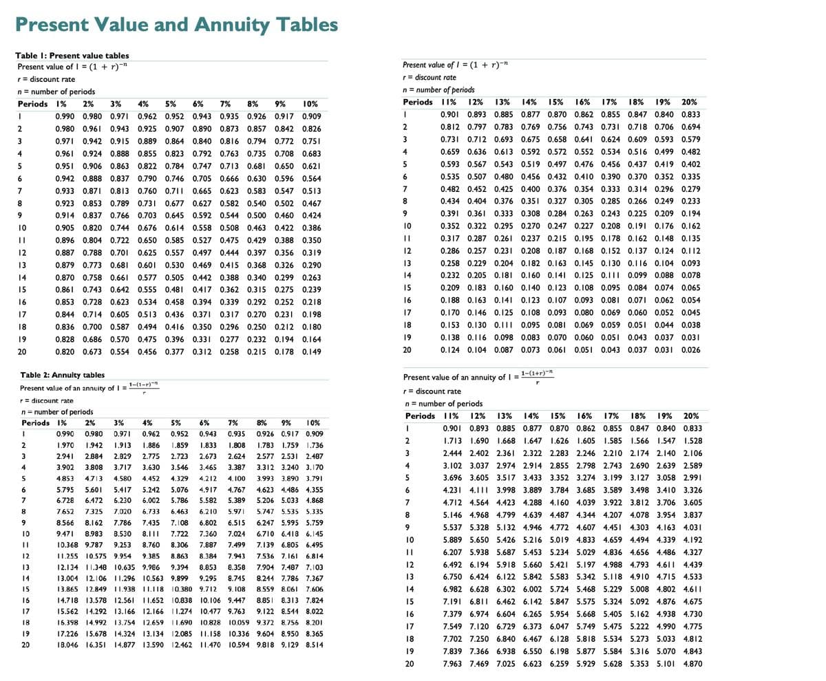
Present Value and Annuity Tables Table I: Present value tables Present value of I = (1 + r)¯" Present value of I = (1 + r)¯n r = discount rate r= discount rate n = number of periods n = number of periods Periods 1% 2% 3% 4% 5% 6% 7% 8% 9% 10% Periods I1% 1 2% 13% 14% 1% 16% 17% 18% 19% 20% 0.990 0.980 0.971 0.962 0.952 0.943 0.935 0.926 0.917 0.909 0.901 0.893 0.885 0.877 0.870 0.862 0.855 0.847 0.840 0.833 0.980 0.961 0.943 0.925 0.907 0.890 0.873 0.857 0.842 0.826 2 0.812 0.797 0.783 0.769 0.756 0.743 0.731 0.718 0.706 0.694 3 0.971 0.942 0.915 0.889 0.864 0.840 0.816 0.794 0.772 0.751 3 0.731 0.712 0.693 0.675 0.658 0.641 0.624 0.609 0.593 0.579 4 0.961 0.924 0.888 0.855 0.823 0.792 0.763 0.735 0.708 0.683 4 0.659 0.636 0.613 0.592 0.572 0.552 0.534 0.516 0.499 0.482 0.951 0.906 0.863 0.822 0.784 0.747 0.713 0.681 0.650 0.621 5 0.593 0.567 0.543 0.519 0.497 0.476 0.456 0.437 0.419 0.402 6 0.942 0.888 0.837 0.790 0.746 0.705 0.666 0.630 0.596 0.564 6 0.535 0.507 0.480 0.456 0.432 0.410 0.390 0.370 0.352 0.335 7 0.933 0.871 0.813 0.760 0.71| 0.665 0.623 0.583 0.547 0.513 7 0.482 0.452 0.425 0.400 0.376 0.354 0.333 0.314 0.296 0.279 8 0.923 0.853 0.789 0.731 0.677 0.627 0.582 0.540 0.502 0.467 8. 0.434 0.404 0.376 0.351 0.327 0.305 0.285 0.266 0.249 0.233 9 0.914 0.837 0.766 0.703 0.645 0.592 0.544 0.500 0.460 0.424 9 0.391 0.361 0.333 0.308 0.284 0.263 0.243 0.225 0.209 0.194 10 0.905 0.820 0.744 0.676 0.614 0.558 0.508 0.463 0.422 0.386 10 0.352 0.322 0.295 0.270 0.247 0.227 0.208 0.191 0.176 0.162 0.896 0.804 0.722 0.650 0.585 0.527 0.475 0.429 0.388 0.350 || 0.317 0.287 0.261 0.237 0.215 0.195 0.178 0.162 0.148 0.135 12 0.887 0.788 0.701 0.625 0.557 0.497 0.444 0.397 0.356 0.319 12 0.286 0.257 0.231 0.208 0.187 0.168 0.152 0.137 0.124 0.112 13 0.879 0.773 0.681 0.601 0.530 0.469 0.415 0.368 0.326 0.290 13 0.258 0.229 0.204 0.182 0.163 0.145 0.130 0.116 0.104 0.093 14 0.870 0.758 0.661 0.577 0.505 0.442 0.388 0.340 0.299 0.263 14 0.232 0.205 0.181 0.160 0.141 0.125 0.11| 0.099 0.088 0.078 15 0.861 0.743 0.642 0.555 0.481 0.417 0.362 0.315 0.275 0.239 15 0.209 0.183 0.160 0.140 0.123 0.108 0.095 0.084 0.074 0.065 16 0.853 0.728 0.623 0.534 0.458 0.394 0.339 0.292 0.252 0.218 16 0.188 0.163 0.141 0.123 0.107 0.093 0.081 0.071 0.062 0.054 17 0.844 0.714 0.605 0.513 0.436 0.371 0.317 0.270 0.231 0.198 17 0.170 0.146 0.125 0.108 0.093 0.080 0.069 0.060 0.052 0.045 18 0.836 0.700 0.587 0.494 0.416 0.350 0.296 0.250 0.212 0.180 18 0.153 0.130 0.1|I 0.095 0.081 0.069 0.059 0.051 0.044 0.038 19 0.828 0.686 0.570 0.475 0.396 0.331 0.277 0.232 0.194 0.164 19 0.138 0.116 0.098 0.083 0.070 0.060 0.051 0.043 0.037 0.031 20 0.820 0.673 0.554 0.456 0.377 0.312 0.258 0.215 0.178 0.149 20 0.124 0.104 0.087 0.073 0.061 0.051 0.043 0.037 0.031 0.026 Table 2: Annuity tables Present value of an annuity of I = 1-(1+r)-n 1-(1-r)-n Present value of an annuity of = r = discount rate r = discount rate n = number of periods n = number of periods Periods I1% 12% 13% 14% 15% 16% 17% 18% 19% 20% Periods 1% 2% 3% 4% 5% 6% 7% 8% 9% 10% 0.901 0.893 0.885 0.877 0.870 0.862 0.855 0.847 0.840 0.833 0.990 0.980 0.971 0.962 0.952 0.943 0.935 0.926 0.917 0.909 2 1.713 1.690 1.668 1.647 1.626 1.605 1.585 1.566 1.547 1.528 2 1.970 1.942 1.913 1.886 1.859 1.833 1.808 1.783 1.759 1.736 3 2.444 2.402 2.361 2.322 2.283 2.246 2.210 2.174 2.140 2.106 3 2.941 2.884 2.829 2.775 2.723 2.673 2.624 2.577 2.531 2.487 4 3.902 3.808 3.717 3.630 3.546 3.465 3.387 3.312 3.240 3.170 4 3.102 3.037 2.974 2.914 2.855 2.798 2.743 2.690 2.639 2.589 4.853 4.713 4.580 4.452 4.329 4.212 4. 100 3.993 3.890 3.791 3.696 3.605 3.517 3.433 3.352 3.274 3.199 3.127 3.058 2.991 6 5.795 5.601 5.417 5.242 5.076 4.917 4.767 4.623 4.486 4.355 6 4.231 4.111 3.998 3.889 3.784 3.685 3.589 3.498 3.410 3.326 6.728 6.472 6.230 6.002 5.786 5.582 5.389 5.206 5.033 4.868 7 4.712 4.564 4.423 4.288 4.160 4.039 3.922 3.812 3.706 3.605 8 7.652 7.325 7.020 6.733 6.463 6.210 5.97| 5.747 5.535 5.335 8 5.146 4.968 4.799 4.639 4.487 4.344 4.207 4.078 3.954 3.837 9 8.566 8.162 7.786 7.435 7.108 6.802 6.515 6.247 5.995 5.759 5.537 5.328 5.132 4.946 4.772 4.607 4.45I 4.303 4.163 4.031 10 9.471 8.983 8.530 8.111 7.722 7.360 7.024 6.710 6.418 6.145 10 5.889 5.650 5.426 5.216 5.019 4.833 4.659 4.494 4.339 4.192 10.368 9.787 9.253 8.760 8.306 7.887 7.499 7.139 6.805 6.495 || 6.207 5.938 5.687 5.453 5.234 5.029 4.836 4.656 4.486 4.327 12 I1.255 10.575 9.954 9.385 8.863 8.384 7.943 7.536 7.161 6.814 13 12.134 |1.348 10.635 9.986 9.394 8.853 8.358 7.904 7.487 7.103 12 6.492 6.194 5.918 5.660 5.421 5.197 4.988 4.793 4.6|| 4.439 14 13.004 12.106 11.296 10.563 9.899 9.295 8.745 8.244 7.786 7.367 13 6.750 6.424 6.122 5.842 5.583 5.342 5.118 4.910 4.715 4.533 15 13.865 12.849 11.938 II.118 10.380 9.712 9. 108 8.559 8.06I 7.606 14 6.982 6.628 6.302 6.002 5.724 5.468 5.229 5.008 4.802 4.61| 16 14.718 13.578 12.561 11.652 10.838 10.106 9.447 8.85 8.313 7.824 15 7.191 6.811 6.462 6.142 5.847 5.575 5.324 5.092 4.876 4.675 17 15.562 14.292 13.166 12.166 I1.274 10.477 9.763 9.122 8.544 8.022 16 7.379 6.974 6.604 6.265 5.954 5.668 5.405 5.162 4.938 4.730 18 16.398 14.992 13.754 12.659 |1.690 10.828 10.059 9.372 8.756 8.201 17 7.549 7.120 6.729 6.373 6.047 5.749 5.475 5.222 4.990 4.775 19 17.226 15.678 14.324 13.134 12.085 11.158 10.336 9.604 8.950 8.365 18 7.702 7.250 6.840 6.467 6.128 5.818 5.534 5.273 5.033 4.812 20 18.046 16.351 14.877 13.590 12.462 |1.47O 10.594 9.818 9.129 8.514 19 7.839 7.366 6.938 6.550 6.198 5.877 5.584 5.316 5.070 4.843 20 7.963 7.469 7.025 6.623 6.259 5.929 5.628 5.353 5.101 4.870 Financial ratios Creditors days Working capital Cost of capital Gross margin (%) Economic order quantity (EOQ) Cost of equity Trade payables Gross profit x 365 Purchases × 100 2DC ke = Do(1+g) + g Po Revenue or H Operating margin (%) Trade creditors or Operating profit x 100 x 365 Cash management (1) Purchases ke = R, + B(Rm – R;) Revenue If 'Purchases' figure not available, use 'Cost of sales 2NF Z = Return on capital employed (%) Financial gearing (%) WACC Cash management (2) Ve ke: Ve+Va Va + ka (1 – t) Operating profit x 100 Long-term debt Shareholders equity + Long-term debt x 100 Ve+Va Long-term debt + Shareholders equity Return on equity (%) S = 3 Parity theory Interest cover (times) Operating profit Interest charges Profit after taxation x 100 Learning curve PPPT Shareholders equity (1+ir) Return on total assets (%) y = axb S1 = So (1+in) Earnings per share (EPS) Profit after taxation Variances x 100 IRPT Profit after taxation Total assets Number of ordinary shares in issue Sales price (1+if) Asset turnover Price I earnings ratio (PIE) (Actual selling price – Budgeted selling price) x Actual units sold Fo = So (1+in) Revenue Share price Financial arithmetic Total assets Sales volume Earnings per share Current ratio (Actual units sold – Budgeted quantity) x Budgeted contribution per unit Effective annual rate of interest Earnings yield Current assets Material price [1+"-1 Current liabilities Earnings per share Quick test (acid ratio) (Budgeted cost – Actual cost) x Actual quantity used Share price Present value of I Current assets - Inventory Dividend per share (DPS) Material usage [1+ r]-" Present value of an annuity of I Current liabilities Total dividends for the period (Budgeted quantity – Actual quantity) x Budgeted cost per unit Working capital turnover Number of ordinary shares in issue Labour rate Revenue Dividend cover 1-(1+r)-" Net working capital (Budgeted rate – Actual rate) x Actual time taken Profit after taxation Inventory turnover Labour efficiency Total dividends for the period (Budgeted time - Actual time taken) x Budgeted rate Cost of sales Dividend payout (%) Inventory Total dividends for the period Variable overhead rate Inventory days x 100 Profit after taxation (Budgeted rate – Actual rate) x Actual time taken Inventory x 365 or Cost of sales Variable overhead efficiency DPS Debtors days × 100 (Budgeted time - Actual time taken) x Budgeted rate EPS Dividend yield Trade receivables x 365 Fixed overhead expenditure Revenue Dividend per share (Budgeted fixed overhead – Actual fixed overhead) or Share price Trade debtors x 365 Revenue

The following information relates to a proposed four-year project which is being financially evaluated by the Board of Directors of Pampass Inc. (Pampass). Pampass is an unlisted company but shareholders include private investors, a venture capital company, an insurance company and a pension fund. The initial investment is $7.8 million, with scrap value of $0.2 million and the following net cash inflows for each of the four years:

The Board of Directors believes that this project will increase shareholder wealth if it achieves an accounting rate of return (ARR) greater than 20%. As a matter of policy, the Board requires all investment projects to be evaluated using both ARR and payback period. Shareholders have recently criticised the Board of Directors for using these investment appraisal methods, claiming that Pampass should be using the net present value method. The directors’ remuneration package includes a financial reward for achieving an ARR greater than 20% but does not include a share option scheme.

Required:

1. What is the payback period of the proposed project?

1. What is the average rate of return (ARR) of the proposed project?

1. Which of the following statements about investment appraisal methods is/are not correct?

1. ARR must be greater than the cost of equity if a project is to be accepted
2. Riskier projects should be evaluated with longer payback periods
3. The ARR method does not consider the time value of money

1. Which of the following statements about Pampass is/are correct?

1. Managerial reward schemes should not encourage the achievement of stakeholderobjectives
2. Requiring investment projects to be evaluated via the ARR method is an example of dysfunctional behaviour encouraged by performance-related pay
3. Pampass does not have an agency problem as the Board of Directors is acting to maximise shareholder wealth

1. Which of the following statements is/are not correct?

1. Introducing a share option scheme in Pampass would help bring directors’ objectives in line with shareholders’ objectives
2. By linking their financial rewards to a target ARR, Pampass is encouraging its directors to focus on short-term profitability and discouraging them to make long-term capital investment decisions
3. Directors’ remuneration in Pampass should be determined by its senior executive directors