Many small restaurants in Portland, Oregon, and other cities across the United States do not take reservations. Owners say that with smaller capacity, noshows are costly, and they would rather have their staff focused on customer service rather than maintaining a reservation system (pressherald.com). However, it is important to be able to give reasonable estimates of waiting time when customers arrive and put their name on the waiting list. The file RestaurantLine contains 10 observations of number of people in line ahead of a customer (independent variable x) and actual waiting time (dependent variable y). The estimated regression equation is: ŷ=11.97+7.68x and MSE=144.2066. Use Table 2 of Appendix B. a. Develop a point estimate for a customer who arrive with three people on the wait-list (to 1 decimal). b. Develop a confidence interval for the mean waiting time for a customer who arrives with three customers already in line (to 2 decimals). c. Develop a prediction interval for Roger


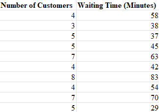
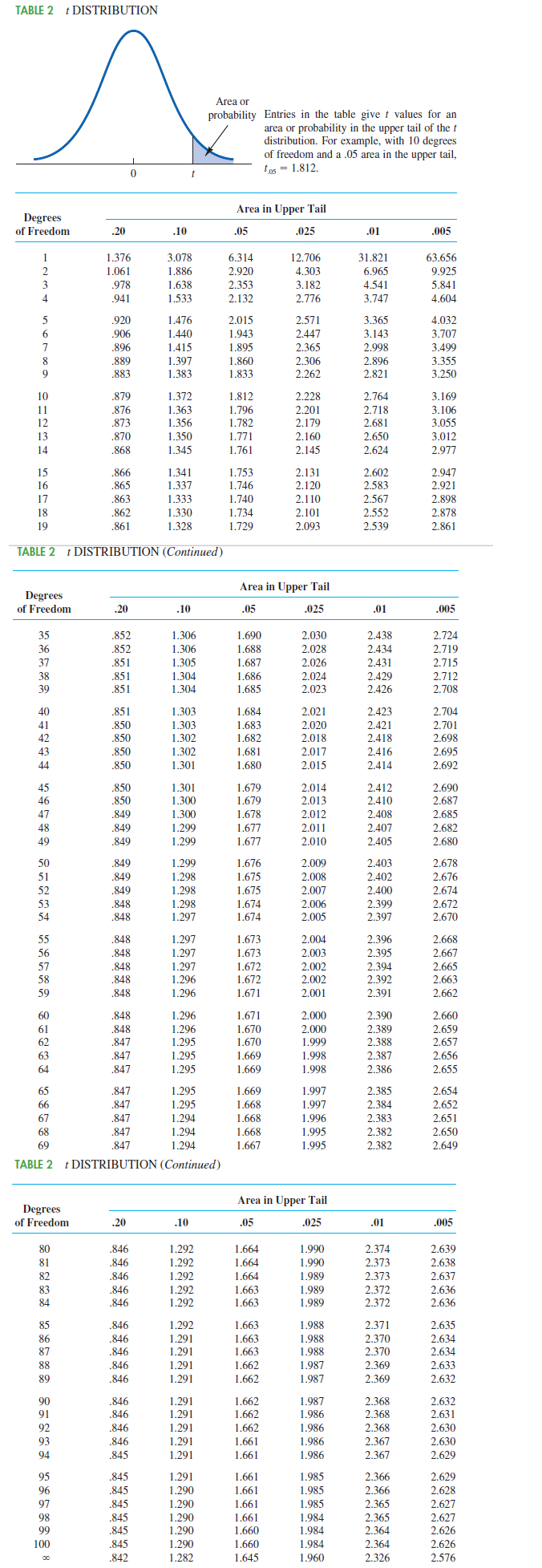
Many small restaurants in Portland, Oregon, and other cities across the United States do not take reservations. Owners say that with smaller capacity, noshows are costly, and they would rather have their staff focused on customer service rather than maintaining a reservation system (pressherald.com). However, it is important to be able to give reasonable estimates of waiting time when customers arrive and put their name on the waiting list. The file RestaurantLine contains 10 observations of number of people in line ahead of a customer (independent variable x) and actual waiting time (dependent variable y). The estimated regression equation is: ŷ=11.97+7.68x and MSE=144.2066. Use Table 2 of Appendix B.
a. Develop a point estimate for a customer who arrive with three people on the wait-list (to 1 decimal).
b. Develop a confidence interval for the mean waiting time for a customer who arrives with three customers already in line (to 2 decimals).
c. Develop a prediction interval for Roger and Sherry Davy's waiting time if there are three customers in line when they arrive (to 2 decimals).

Step by step
Solved in 4 steps with 4 images


