Plant spacing can have both a positive and negative effect on crop yield. For example, closer spacing increases the number of plants and hence the yield per acre, but it also increases plant competition for available nutrients and moisture, thereby reducing the yield per plant. For an investigation of the effect of raw spacing on the production of garden peas, equal-sized fields at seven different locations were available. At each location, the field was divided into three square, equal- sized plots. Peas were planted at each location by randomly assigning one plot to be sown in a 4 inch row spacing, a second plot to be sown in an 8 inch row spacing and the third plot to be sown in a 12 inch row spacing. All plots were planted on the same date, and the plots at each location were treated the same except for row spacing. The yields of peas in bushels/ acre for each plot is given in the data table. The image below provide the following details : (1) Table on the left represents yield of a crop taken from 7 different locations. Row spacing denotes the spacing of plants. From each location, three different yield values are taken with 3 different plant spacing (2) The table on the right provides summary statistics of each sample based on the 'row-spacing'. How do we select the best(optimal) plant spacing for this crop, by interpreting the summary statistics of the table?


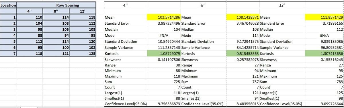
Plant spacing can have both a positive and negative effect on crop yield. For example, closer spacing increases the number of plants and hence the yield per acre, but it also increases plant competition for available nutrients and moisture, thereby reducing the yield per plant. For an investigation of the effect of raw spacing on the production of garden peas, equal-sized fields at seven different locations were available. At each location, the field was divided into three square, equal- sized plots. Peas were planted at each location by randomly assigning one plot to be sown in a 4 inch row spacing, a second plot to be sown in an 8 inch row spacing and the third plot to be sown in a 12 inch row spacing. All plots were planted on the same date, and the plots at each location were treated the same except for row spacing. The yields of peas in bushels/ acre for each plot is given in the data table.
The image below provide the following details :
(1) Table on the left represents yield of a crop taken from 7 different locations. Row spacing denotes the spacing of plants. From each location, three different yield values are taken with 3 different plant spacing
(2) The table on the right provides summary statistics of each sample based on the 'row-spacing'.
How do we select the best(optimal) plant spacing for this crop, by interpreting the summary statistics of the table?
Can I have a step-by-step explanation on that?
Thank you!


Trending now
This is a popular solution!

Step by step
Solved in 2 steps


