Please show me step by step following tables, identify the test, interpret the results and report them in an academic s
Please show me step by step following tables, identify the test, interpret the results and report them in an academic s

MATLAB: An Introduction with Applications
6th Edition
ISBN:9781119256830
Author:Amos Gilat
Publisher:Amos Gilat
Chapter1: Starting With Matlab
Section: Chapter Questions
Problem 1P

Related questions
Question
Please please how to write if based on the following tables, identify the test, interpret the results and report them in an academic style. So do not need to interpret the assumptions. Please show me step by step following tables, identify the test, interpret the results and report them in an academic style.
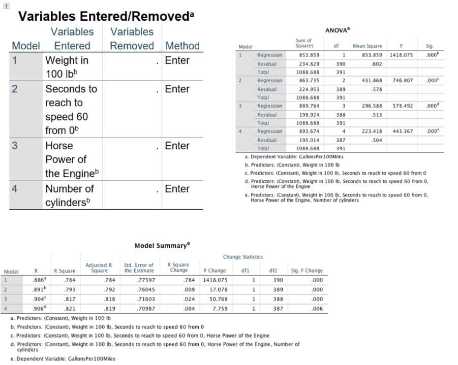
Transcribed Image Text:Variables Entered/Removeda
Variables Variables
Model Entered Removed Method
1
. Enter
2
3
4
Model
1
2
Weight in
100 lbb
Seconds to
reach to
speed 60
from 0b
Horse
Power of
the Engineb
Number of
cylindersb
R
.886
.891b
.904€
.906d
R Square
.784
.793
.817
.821
Adjusted R
Square
Std. Error of
the Estimate
.
77597
.76045
.71603
.70987
Enter
Enter
Model Summary
Enter
R Square
Change
784
.009
.024
.004
Model
1 Regression
Residual
Total
F Change
1418.075
17.078
50.768
7.759
3
Change Statistics
dfl
1
1
1
1
Sum of
Squares
853.859
234.829
1088.688
863.735
224.953
1088.688
889.764
198.924
1088.688
893.674
1
390
391
2 Regression
2
389
391
Residual
Total
Regression
Residual
Total
Regression
Residual
3
388
391
4
387
195.014
Total
1088.688
391
a. Dependent Variable: GallonsPer 100 Miles
b. Predictors: (Constant), Weight in 100 lb
c. Predictors: (Constant), Weight in 100 lb, Seconds to reach to speed 60 from 0
d. Predictors: (Constant), Weight in 100 lb, Seconds to reach to speed 60 from 0.
Horse Power of the Engine
df2
390
389
388
387
ANOVA
Sig. F Change
.000
.000
.000
.006
df
.784
.792
.816
.819
a. Predictors: (Constant), Weight in 100 lb
b. Predictors: (Constant), Weight in 100 lb. Seconds to reach to speed 60 from 0
c. Predictors: (Constant), Weight in 100 lb, Seconds to reach to speed 60 from 0, Horse Power of the Engine
d. Predictors: (Constant), Weight in 100 lb, Seconds to reach to speed 60 from 0, Horse Power of the Engine, Number of
cylinders
e. Dependent Variable: GallonsPer100Miles
Mean Square
853.859
.602
F
1418.075
431.868 746.807
.578
296.588
513
223.418
.504
e. Predictors: (Constant), Weight in 100 lb, Seconds to reach to speed 60 from 0.
Horse Power of the Engine, Number of cylinders
Sig.
.000
578.492
.000€
.000⁰
443.367 .000*
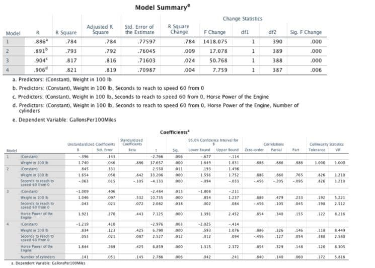
Transcribed Image Text:Model
1
2
3
Model
1
2
3
R
.886
.891b
-904€
.906
(Constant
Weight in 100 b
(Constant
Weight in 100 b
Seconds to reach to
speed 60 from 0
Constant
Weight in 100 b
Seconds to reach to
speed 60 from 0
Horse Power of the
Engine
R Square
.784
.793
.817
.821
(Constant
Weight in 100 b
Seconds to reach to
speed 60 from 0
Adjusted R
Square
Unstandardized Coefficients
Std. Error
-.396
1.740
845
1.654
-.063
-1.009
1.046
.043
1.921
-1.219
834
.053
.784
.792
.816
.819
Horse Power of the
Engine
Number of cylinders
141
a. Dependent Variable: GallonsPer 100 Miles
a. Predictors: (Constant), Weight in 100 lb
b. Predictors: (Constant), Weight in 100 lb. Seconds to reach to speed 60 from 0
c. Predictors: (Constant), Weight in 100 lb. Seconds to reach to speed 60 from 0, Horse Power of the Engine
d. Predictors: (Constant), Weight in 100 lb, Seconds to reach to speed 60 from 0, Horse Power of the Engine, Number of
cylinders
e. Dependent Variable: GallonsPer 100Miles
1.844
-143
046
331
050
015
406
097
021
270
410
123
021
269
Model Summary
051
Std. Error of
the Estimate
.77597
.76045
.71603
.70987
Standardized
Coefficients
Beta
1
-2.766
886 37.657
2.550
33.206
-4.133
842
-105
-2.484
10.735
532
072 2.082
Coefficients
443 7.125
-2.976
6.790
2.527
425
087
425 6.859
145
R Square
Change
2.786
.784
.009
.024
.004
Sig.
006
000
011
000
000
013
.000
038
000
003
000
012
000
006
F Change df1
1418.075
17.078
50.768
7.759
Change Statistics
95.0% Confidence Interval for
Lower Bound Upper Bound
-677
-114
1.649
1.831
193
1.496
1.556
1.752
-.094
-.033
-1.808
854
.002
1.391
-2.025
593
2012
1.315
042
-211
1.237
084
2.452
-414
1.076
094
2.372
1
1
1
1
241
886
Correlations
Zero-order Partial
885
-456
854
df2
886
-456
390
389
388
387
.854
840
.886
860
765
-456 -205 -.095
886
479
105
340
326
127
Sig. F Change
.000
.000
.000
.006
329
140
Collinearity Statistics
Part Tolerance
VIF
886
233
045
155
146
054
148
060
1.000
826
826
192
398
122
120
1.000
172
1.210
1.210
5.221
2.312
118 8.449
388
2.580
8.216
8.305
5.816
Expert Solution
This question has been solved!
Explore an expertly crafted, step-by-step solution for a thorough understanding of key concepts.

Step by step
Solved in 3 steps with 1 images

Recommended textbooks for you
MATLAB: An Introduction with Applications
Statistics
ISBN:
9781119256830
Author:
Amos Gilat
Publisher:
John Wiley & Sons Inc

Probability and Statistics for Engineering and th…
Statistics
ISBN:
9781305251809
Author:
Jay L. Devore
Publisher:
Cengage Learning

Statistics for The Behavioral Sciences (MindTap C…
Statistics
ISBN:
9781305504912
Author:
Frederick J Gravetter, Larry B. Wallnau
Publisher:
Cengage Learning
MATLAB: An Introduction with Applications
Statistics
ISBN:
9781119256830
Author:
Amos Gilat
Publisher:
John Wiley & Sons Inc
Probability and Statistics for Engineering and th…
Statistics
ISBN:
9781305251809
Author:
Jay L. Devore
Publisher:
Cengage Learning
Statistics for The Behavioral Sciences (MindTap C…
Statistics
ISBN:
9781305504912
Author:
Frederick J Gravetter, Larry B. Wallnau
Publisher:
Cengage Learning

Elementary Statistics: Picturing the World (7th E…
Statistics
ISBN:
9780134683416
Author:
Ron Larson, Betsy Farber
Publisher:
PEARSON

The Basic Practice of Statistics
Statistics
ISBN:
9781319042578
Author:
David S. Moore, William I. Notz, Michael A. Fligner
Publisher:
W. H. Freeman

Introduction to the Practice of Statistics
Statistics
ISBN:
9781319013387
Author:
David S. Moore, George P. McCabe, Bruce A. Craig
Publisher:
W. H. Freeman