Problem 3. Performance data for a pump are given in the table below. From a curve fit to the data, the pump curve is given by H, = H, – C, Q² whereHo = 180 ft and C, = 1.524 × 10⁻⁶ ft/gpm?. This pump is used to move water at STP between two open reservoirs with an elevation increase of Az = 50 ft through a commercial steel pipe of length L = 1200 ft and diameter D = 1.0 ft that contains two 90° elbows (equivalent length of 30 diameters) and an open gate valve (equivalent length of 8 diameters). The flow entrance and exit for the reservoirs are abrupt. (a) Plot the pump curve and system curve on the same figure. (b) Calculate the flowrate with the gate valve open. (c) Calculate the equivalent length for the gate valve in order to reduce the flowrate by half. NOTE: Your calculations for this problem will require iteration because the friction factor for this case does depend on Q. Thus, it is recommended you use either EES (see solution for Example 19 from lecture) or Excel to get converged values. Q (gpm) Н, (ft) 500 1000 1500 2000 2500 3000 179 176 165 145 119 84 43
Problem 3. Performance data for a pump are given in the table below. From a curve fit to the data, the pump curve is given by H, = H, – C, Q² whereHo = 180 ft and C, = 1.524 × 10⁻⁶ ft/gpm?. This pump is used to move water at STP between two open reservoirs with an elevation increase of Az = 50 ft through a commercial steel pipe of length L = 1200 ft and diameter D = 1.0 ft that contains two 90° elbows (equivalent length of 30 diameters) and an open gate valve (equivalent length of 8 diameters). The flow entrance and exit for the reservoirs are abrupt. (a) Plot the pump curve and system curve on the same figure. (b) Calculate the flowrate with the gate valve open. (c) Calculate the equivalent length for the gate valve in order to reduce the flowrate by half. NOTE: Your calculations for this problem will require iteration because the friction factor for this case does depend on Q. Thus, it is recommended you use either EES (see solution for Example 19 from lecture) or Excel to get converged values. Q (gpm) Н, (ft) 500 1000 1500 2000 2500 3000 179 176 165 145 119 84 43

Elements Of Electromagnetics
7th Edition
ISBN:9780190698614
Author:Sadiku, Matthew N. O.
Publisher:Sadiku, Matthew N. O.
ChapterMA: Math Assessment
Section: Chapter Questions
Problem 1.1MA

Related questions

Question
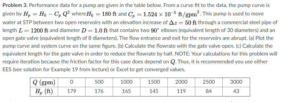
Transcribed Image Text:Problem 3. Performance data for a pump are given in the table below. From a curve fit to the data, the pump curve is
given by Hp
= Ho – C, Q² where Ho = 180 ft and C, = 1.524 × 10⁻⁵ ft/gpm?. This pump is used to move
water at STP between two open reservoirs with an elevation increase of Az = 50 ft through a commercial steel pipe of
length L = 1200 ft and diameter D = 1.0 ft that contains two 90° elbows (equivalent length of 30 diameters) and an
open gate valve (equivalent length of 8 diameters). The flow entrance and exit for the reservoirs are abrupt. (a) Plot the
pump curve and system curve on the same figure. (b) Calculate the flowrate with the gate valve open. (c) Calculate the
equivalent length for the gate valve in order to reduce the flowrate by half. NOTE: Your calculations for this problem will
require iteration because the friction factor for this case does depend on Q. Thus, it is recommended you use either
EES (see solution for Example 19 from lecture) or Excel to get converged values.
Q (gpm)
H, (ft)
500
1000
1500
2000
2500
3000
179
176
165
145
119
84
43
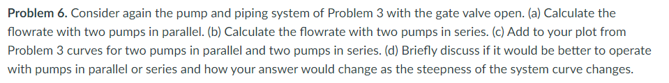
Transcribed Image Text:Problem 6. Consider again the pump and piping system of Problem 3 with the gate valve open. (a) Calculate the
flowrate with two pumps in parallel. (b) Calculate the flowrate with two pumps in series. (c) Add to your plot from
Problem 3 curves for two pumps in parallel and two pumps in series. (d) Briefly discuss if it would be better to operate
with pumps in parallel or series and how your answer would change as the steepness of the system curve changes.
Expert Solution
This question has been solved!
Explore an expertly crafted, step-by-step solution for a thorough understanding of key concepts.

This is a popular solution!

Trending now
This is a popular solution!

Step by step
Solved in 3 steps with 2 images

Knowledge Booster


Learn more about
Need a deep-dive on the concept behind this application? Look no further. Learn more about this topic, mechanical-engineering and related others by exploring similar questions and additional content below.Recommended textbooks for you
Elements Of Electromagnetics
Mechanical Engineering
ISBN:
9780190698614
Author:
Sadiku, Matthew N. O.
Publisher:
Oxford University Press

Mechanics of Materials (10th Edition)
Mechanical Engineering
ISBN:
9780134319650
Author:
Russell C. Hibbeler
Publisher:
PEARSON

Thermodynamics: An Engineering Approach
Mechanical Engineering
ISBN:
9781259822674
Author:
Yunus A. Cengel Dr., Michael A. Boles
Publisher:
McGraw-Hill Education
Elements Of Electromagnetics
Mechanical Engineering
ISBN:
9780190698614
Author:
Sadiku, Matthew N. O.
Publisher:
Oxford University Press
Mechanics of Materials (10th Edition)
Mechanical Engineering
ISBN:
9780134319650
Author:
Russell C. Hibbeler
Publisher:
PEARSON
Thermodynamics: An Engineering Approach
Mechanical Engineering
ISBN:
9781259822674
Author:
Yunus A. Cengel Dr., Michael A. Boles
Publisher:
McGraw-Hill Education

Control Systems Engineering
Mechanical Engineering
ISBN:
9781118170519
Author:
Norman S. Nise
Publisher:
WILEY

Mechanics of Materials (MindTap Course List)
Mechanical Engineering
ISBN:
9781337093347
Author:
Barry J. Goodno, James M. Gere
Publisher:
Cengage Learning

Engineering Mechanics: Statics
Mechanical Engineering
ISBN:
9781118807330
Author:
James L. Meriam, L. G. Kraige, J. N. Bolton
Publisher:
WILEY