Problems 1 - 4 share the same summaries presented in the table below. Two groups of students,graduates and undergraduates, were subject to comparative studies. Their individual grades are assumedto be normal with unknown parameters.Respondents were selected independently and their sample summaries are presented in the table below.GroupSizeMean = XVariance = S?V =Graduateni = 10 | (X)1= 85.1(S2)1 = 40vị =4600Undergraduate n2 = 10 (X)2 = 70.9(S²)2 = 600V2 =10= 60For all hypothesis testing problems, you are supposed to show your conclusions in the standardized formas follows.1. Test statistic value2. Critical values required3. State rejection rule explaining what you decide4. The decision such as "yes, reject the null" or "not enough evidence for rejection"Deriving confidence intervals, please show critical values needed and present your interval in the formUCL =LCL = Continue with the same summaries and assumption as in Problem 3.Faculty assumed that two populations have ENTIRELY UNKNOWN VARIANCES, (01)² and (02)².Samples of size nį = n2 = n = 10 were collected and summarized, with summaries presented in the tableshown on page 2.Estimate the difference, u = µ1 – µ2 between two population means with confidence C = 0.95.1. Show critical value (or values) needed for this procedure2. Evaluate upper and lower confidence limits for the targeted parameter, µ1 – 2.

Answered: Problems 1 - 4 share the same summaries…

MATLAB: An Introduction with Applications

6th Edition

ISBN:9781119256830

Author:Amos Gilat

Publisher:Amos Gilat

Chapter1: Starting With Matlab

Section: Chapter Questions

Problem 1P

See similar textbooks

Related questions

Concept explainers

Question

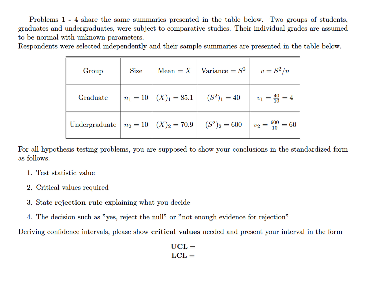
Problems 1 - 4 share the same summaries presented in the table below. Two groups of students,
graduates and undergraduates, were subject to comparative studies. Their individual grades are assumed
to be normal with unknown parameters.
Respondents were selected independently and their sample summaries are presented in the table below.
Group
Size
Mean = X
Variance = S?
V =
Graduate
ni = 10 | (X)1= 85.1
(S2)1 = 40
vị =
4
600
Undergraduate n2 = 10 (X)2 = 70.9
(S²)2 = 600
V2 =
10
= 60
For all hypothesis testing problems, you are supposed to show your conclusions in the standardized form
as follows.
1. Test statistic value
2. Critical values required
3. State rejection rule explaining what you decide
4. The decision such as "yes, reject the null" or "not enough evidence for rejection"
Deriving confidence intervals, please show critical values needed and present your interval in the form
UCL =
LCL =

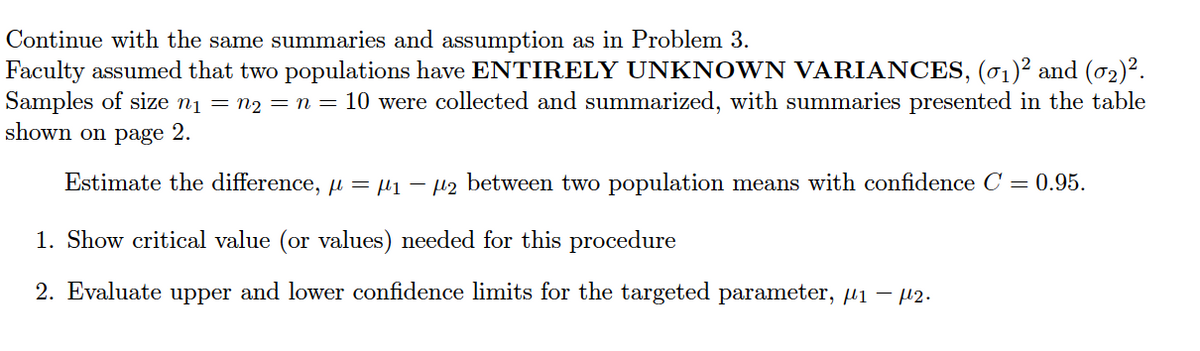
Continue with the same summaries and assumption as in Problem 3.
Faculty assumed that two populations have ENTIRELY UNKNOWN VARIANCES, (01)² and (02)².
Samples of size nį = n2 = n = 10 were collected and summarized, with summaries presented in the table
shown on page 2.
Estimate the difference, u = µ1 – µ2 between two population means with confidence C = 0.95.
1. Show critical value (or values) needed for this procedure
2. Evaluate upper and lower confidence limits for the targeted parameter, µ1 – 2.

Expert Solution

Step 1

Hey, since there are multiple subparts posted, we will answer first three question. If you want any specific question to be answered then please submit that question only or specify the question number in your message.

The test statistic is 1.775, which is obtained below:

$\begin{array}{rcl} t & = & \frac{{\bar{x}}_{1} - {\bar{x}}_{2}}{\sqrt{\frac{s_{1}^{2}}{n_{1}} + \frac{s_{2}^{2}}{n_{2}}}} \\ = & \frac{85.1 - 70.9}{\sqrt{4 + 60}} \\ = & 1.775 \end{array}$

The degrees of freedom is,

$\begin{array}{rcl} d f & = & s m a l l e r o f (n 1 - 1) (n 2 - 1) \\ = & 10 - 1 \\ = & 9 \end{array}$

The critical-value is obtained by using Excel function “=TINV(probability, degrees of freedom)”.

Output obtained from Excel is given below:

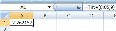
From the output, the critical value for two tailed test with 0.05 level is 2.262.

Step by step

Solved in 2 steps with 1 images

Knowledge Booster

$Point Estimation, Limit Theorems, Approximations, and Bounds$

Learn more about

Need a deep-dive on the concept behind this application? Look no further. Learn more about this topic, statistics and related others by exploring similar questions and additional content below.

Similar questions