Question 6 (For question 6, just write down the answer. No explanation is needed.) (a) Sam and Peter are classmates. In an examination, Sam gets 75 marks and Peter gets 89 marks. It is known that the standard normal score of Sam's marks is 0, z(Sam) = 0 and the standard normal score of Peter's marks is 1.75, z(Peter) = 1.75. Find the standard deviation of the examination marks.
Question 6 (For question 6, just write down the answer. No explanation is needed.) (a) Sam and Peter are classmates. In an examination, Sam gets 75 marks and Peter gets 89 marks. It is known that the standard normal score of Sam's marks is 0, z(Sam) = 0 and the standard normal score of Peter's marks is 1.75, z(Peter) = 1.75. Find the standard deviation of the examination marks.

MATLAB: An Introduction with Applications
6th Edition
ISBN:9781119256830
Author:Amos Gilat
Publisher:Amos Gilat
Chapter1: Starting With Matlab
Section: Chapter Questions
Problem 1P

Related questions
Question
please urgently !!! Correct answer to 4 decimal places and report the measurement unit when applicable.
Transcribed Image Text:Elementary Statistics
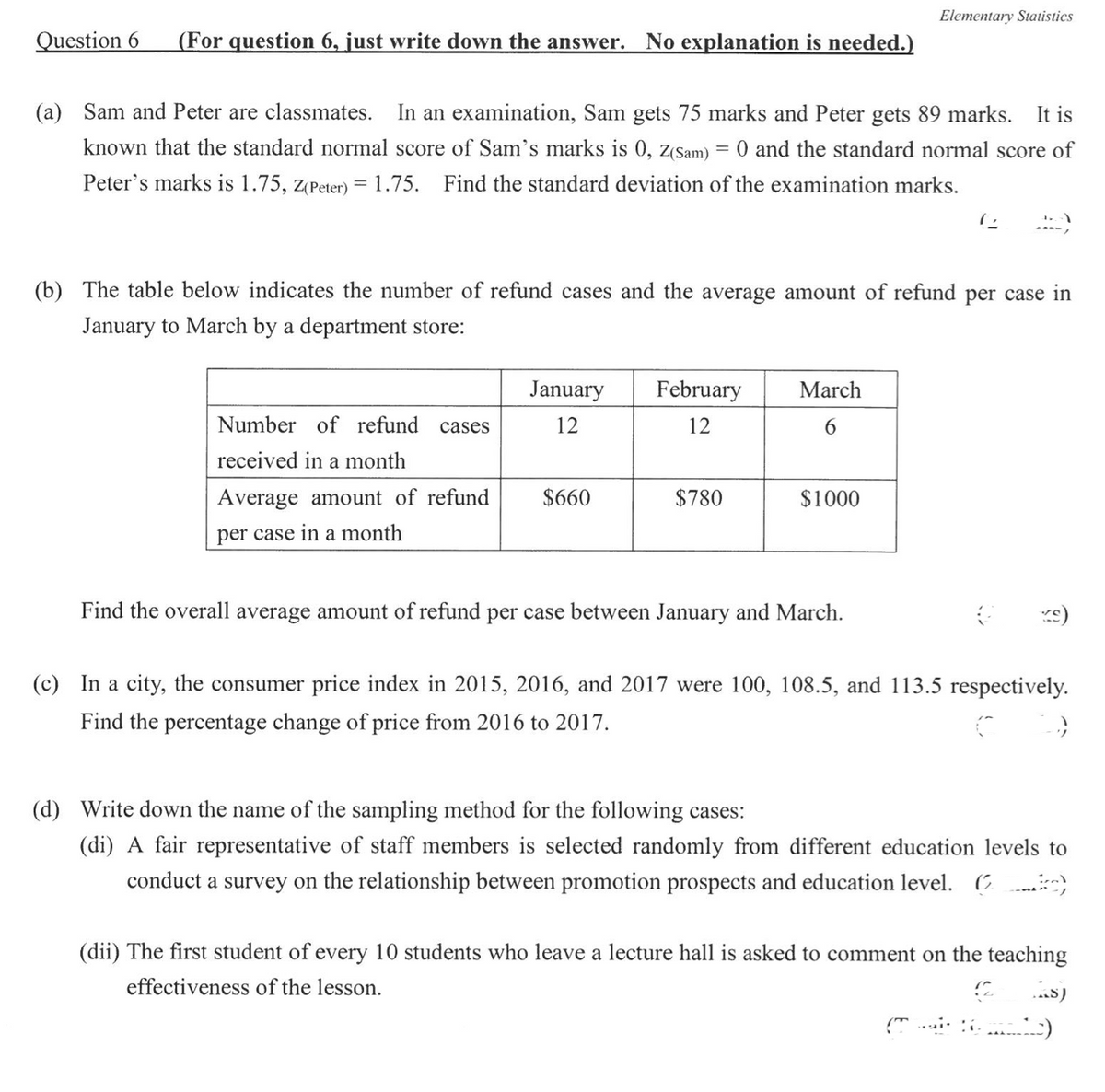
Question 6
(For question 6, just write down the answer.
No explanation is needed.)
(a) Sam and Peter are classmates. In an examination, Sam gets 75 marks and Peter gets 89 marks. It is
known that the standard normal score of Sam's marks is 0, z(Sam) = 0 and the standard normal score of
Peter's marks is 1.75, z(Peter) = 1.75. Find the standard deviation of the examination marks.
(b) The table below indicates the number of refund cases and the average amount of refund per case in
January to March by a department store:
January
February
March
Number of refund
cases
12
12
6.
received in a month
Average amount of refund
$660
$780
$1000
per case in a month
Find the overall average amount of refund per case between January and March.
(c) In a city, the consumer price index in 2015, 2016, and 2017 were 100, 108.5, and 113.5 respectively.
Find the percentage change of price from 2016 to 2017.
(d) Write down the name of the sampling method for the following cases:
(di) A fair representative of staff members is selected randomly from different education levels to
conduct a survey on the relationship between promotion prospects and education level. (2 }
(dii) The first student of every 10 students who leave a lecture hall is asked to comment on the teaching
effectiveness of the lesson.
Transcribed Image Text:Elementary Statistics
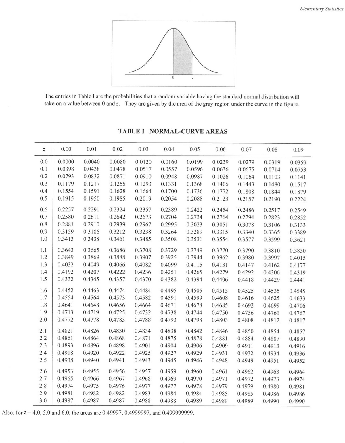
The entries in Table I are the probabilities that a random variable having the standard normal distribution will
take on a value between 0 and z. They are given by the area of the gray region under the curve in the figure.
TABLE I NORMAL-CURVE AREAS
0.00
0.01
0.02
0.03
0.04
0.05
0.06
0.07
0.08
0.09
0.0
0.0000
0.0040
0.0080
0.0120
0.0160
0.0199
0.0239
0.0279
0.0319
0.0359
0.1
0.0398
0.0438
0.0478
0.0517
0.0557
0.0596
0.0636
0.0675
0.0714
0.0753
0.2
0.0793
0.0832
0.0871
0.0910
0.0948
0.0987
0.1026
0.1064
0.1103
0.1141
0.3
0.1179
0.1217
0.1255
0.1293
0.1331
0.1368
0.1406
0.1443
0.1480
0.1517
0.4
0.1554
0.1591
0.1628
0.1664
0.1700
0.1736
0.1772
0.1808
0.1844
0.1879
0.5
0.1915
0.1950
0.1985
0.2019
0.2054
0.2088
0.2123
0.2157
0.2190
0.2224
0.6
0.2257
0.2291
0.2324
0.2357
0.2389
0.2422
0.2454
0.2486
0.2517
0.2549
0.7
0.2580
0.2611
0.2642
0.2673
0.2704
0.2734
0.2764
0.2794
0.2823
0.2852
0.8
0.2881
0.2910
0.2939
0.2967
0.2995
0.3023
0.3051
0.3078
0.3106
0.3133
0.9
0.3159
0.3186
0.3212
0.3238
0.3264
0.3289
0.3315
0.3340
0.3365
0.3389
1.0
0.3413
0.3438
0.3461
0.3485
0.3508
0.3531
0.3554
0.3577
0.3599
0.3621
1.1
0.3643
0.3665
0.3686
0.3708
0.3729
0.3749
0.3770
0.3790
0.3810
0.3830
1.2
0.3849
0.3869
0.3888
0.3907
0.3925
0.3944
0.3962
0.3980
0.3997
0.4015
1.3
0.4032
0.4049
0.4066
0.4082
0.4099
0.4115
0.4131
0.4147
0.4162
0.4177
1.4
0.4192
0.4207
0.4222
0.4236
0.4251
0.4265
0.4279
0.4292
0.4306
0.4319
1.5
0.4332
0.4345
0.4357
0.4370
0.4382
0.4394
0.4406
0.4418
0.4429
0.4441
1.6
0.4452
0.4463
0.4474
0.4484
0.4495
0.4505
0.4515
0.4525
0.4535
0.4545
1.7
0.4554
0.4564
0.4573
0.4582
0.4591
0.4599
0.4608
0.4616
0.4625
0.4633
1.8
0.4641
0.4648
0.4656
0.4664
0.4671
0.4678
0.4685
0.4692
0.4699
0.4706
1.9
0.4713
0.4719
0.4725
0.4732
0.4738
0.4744
0.4750
0.4756
0.4761
0.4767
2.0
0.4772
0.4778
0.4783
0.4788
0.4793
0.4798
0.4803
0.4808
0.4812
0.4817
2.1
0.4821
0.4826
0.4830
0.4834
0.4838
0.4842
0.4846
0.4850
0.4854
0.4857
2.2
0.4861
0.4864
0.4868
0.4871
0.4875
0.4878
0.4881
0.4884
0.4887
0.4890
2.3
0.4893
0.4896
0.4898
0.4901
0.4904
0.4906
0.4909
0.4911
0.4913
0.4916
2.4
0.4918
0.4920
0.4922
0.4925
0.4927
0.4929
0.4931
0.4932
0.4934
0.4936
2.5
0.4938
0.4940
0.4941
0.4943
0.4945
0.4946
0.4948
0.4949
0.4951
0.4952
2.6
0.4953
0.4955
0.4956
0.4957
0.4959
0.4960
0.4961
0.4962
0.4963
0.4964
2.7
0.4965
0.4966
0.4967
0.4968
0.4969
0.4970
0.4971
0.4972
0.4973
0.4974
2.8
0.4974
0.4975
0.4976
0.4977
0.4977
0.4978
0.4979
0.4979
0.4980
0.4981
2.9
0.4981
0.4982
0.4982
0.4983
0.4984
0.4984
0.4985
0.4985
0.4986
0.4986
3.0
0.4987
0.4987
0.4987
0.4988
0.4988
0.4989
0.4989
0.4989
0.4990
0.4990
Also, for z = 4.0, 5.0 and 6.0, the areas are 0.49997, 0.4999997, and 0.499999999.
Expert Solution
This question has been solved!
Explore an expertly crafted, step-by-step solution for a thorough understanding of key concepts.

Step by step
Solved in 2 steps with 2 images

Recommended textbooks for you
MATLAB: An Introduction with Applications
Statistics
ISBN:
9781119256830
Author:
Amos Gilat
Publisher:
John Wiley & Sons Inc

Probability and Statistics for Engineering and th…
Statistics
ISBN:
9781305251809
Author:
Jay L. Devore
Publisher:
Cengage Learning

Statistics for The Behavioral Sciences (MindTap C…
Statistics
ISBN:
9781305504912
Author:
Frederick J Gravetter, Larry B. Wallnau
Publisher:
Cengage Learning
MATLAB: An Introduction with Applications
Statistics
ISBN:
9781119256830
Author:
Amos Gilat
Publisher:
John Wiley & Sons Inc
Probability and Statistics for Engineering and th…
Statistics
ISBN:
9781305251809
Author:
Jay L. Devore
Publisher:
Cengage Learning
Statistics for The Behavioral Sciences (MindTap C…
Statistics
ISBN:
9781305504912
Author:
Frederick J Gravetter, Larry B. Wallnau
Publisher:
Cengage Learning

Elementary Statistics: Picturing the World (7th E…
Statistics
ISBN:
9780134683416
Author:
Ron Larson, Betsy Farber
Publisher:
PEARSON

The Basic Practice of Statistics
Statistics
ISBN:
9781319042578
Author:
David S. Moore, William I. Notz, Michael A. Fligner
Publisher:
W. H. Freeman

Introduction to the Practice of Statistics
Statistics
ISBN:
9781319013387
Author:
David S. Moore, George P. McCabe, Bruce A. Craig
Publisher:
W. H. Freeman