Sketch the sampling distribution and show the area corresponding to the P-value. a -2 O-4 C d (d) Based on your answers in parts (a) to (c), will you reject or fail to reject the null hypothesis? Are the data statistically significant at level a? O At the a = 0.05 level, we reject the null hypothesis and conclude the data are not statistically significant. O At the a = 0.05 level, we fail to reject the null hypothesis and conclude the data are statistically significant. O At the a = 0.05 level, we reject the null hypothesis and conclude the data are statistically significant. O At the a = 0.05 level, we fail to reject the null hypothesis and conclude the data are not statistically significant. (e) State your conclusion in the context of the application. O Fail to reject the null hypothesis, there is sufficient evidence to claim that the mean cost of living index for utilities is less than that for transportation. O Reject the null hypothesis, there is sufficient evidence to claim that the mean cost of living index for utilities is less than that for transportation. O Reject the null hypothesis, there is insufficient evidence to claim that the mean cost of living index for utilities is less than that for transportation. O Fail to reject the null hypothesis, there is insufficient evidence to claim that the mean cost of living index for utilities is less than that for transportation.
Sketch the sampling distribution and show the area corresponding to the P-value. a -2 O-4 C d (d) Based on your answers in parts (a) to (c), will you reject or fail to reject the null hypothesis? Are the data statistically significant at level a? O At the a = 0.05 level, we reject the null hypothesis and conclude the data are not statistically significant. O At the a = 0.05 level, we fail to reject the null hypothesis and conclude the data are statistically significant. O At the a = 0.05 level, we reject the null hypothesis and conclude the data are statistically significant. O At the a = 0.05 level, we fail to reject the null hypothesis and conclude the data are not statistically significant. (e) State your conclusion in the context of the application. O Fail to reject the null hypothesis, there is sufficient evidence to claim that the mean cost of living index for utilities is less than that for transportation. O Reject the null hypothesis, there is sufficient evidence to claim that the mean cost of living index for utilities is less than that for transportation. O Reject the null hypothesis, there is insufficient evidence to claim that the mean cost of living index for utilities is less than that for transportation. O Fail to reject the null hypothesis, there is insufficient evidence to claim that the mean cost of living index for utilities is less than that for transportation.

Glencoe Algebra 1, Student Edition, 9780079039897, 0079039898, 2018
18th Edition
ISBN:9780079039897
Author:Carter
Publisher:Carter
Chapter10: Statistics
Section10.4: Distributions Of Data
Problem 19PFA

Related questions
Topic Video
Question
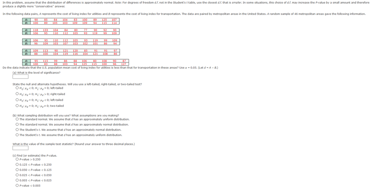
In this problem, assume that the distribution of differences is approximately normal. Note: For degrees of freedom d.f. not in the Student's t table, use the closest d.f. that is smaller. In some situations, this choice of d.f. may increase the P-value by a small amount and therefore produce a slightly more "conservative" answer.
i need help with c, sketching, d and e
Transcribed Image Text:In this problem, assume that the distribution of differences is approximately normal. Note: For degrees of freedom d.f. not in the Student's t table, use the closest d.f. that is smaller. In some situations, this choice of d.f. may increase the P-value by a small amount and therefore
produce a slightly more "conservative" answer.
In the following data pairs, A represents the cost of living index for utilities and B represents the cost of living index for transportation. The data are paired by metropolitan areas in the United States. A random sample of 46 metropolitan areas gave the following information.
A:
B:
90
85
84
104
83
100
89
125
107
100
89
105
103
109
109
94
115
114
A:
В:
118
133
104
84
80
77
90
92
90
106
95
110
112
105
93
119
99
109
A:
106
95
110
112
105
93
119
99
109
B:
96
109
103
107
103
102
101
86
94
A:
B:
109
113
100
90
121
120
85
91
91
97
88
104
119
116
104
121
108
86
90
96
Do the data indicate that the U.S. population mean cost of living index for utilities is less than that for transportation in these areas? Use a = 0.05. (Let d = A - B.)
A:
B:
95
115
99
86
88
106
80
108
87
100
83
103
94
125
115
100
127
(a) What is the level of significance?
State the null and alternate hypotheses. Will you use a left-tailed, right-tailed, or two-tailed test?
O Ho: Hd< 0; H: H= 0; left-tailed
O Ho: Hd = 0; H;: Hd> 0; right-tailed
O Ho: Hd = 0; H;: Hd < 0; left-tailed
O Ho: Hd = 0; H: Hd# 0; two-tailed
(b) What sampling distribution will you use? What assumptions are you making?
O The standard normal. We assume that d has an approximately uniform distribution.
O The standard normal. We assume that d has an approximately normal distribution.
O The Student's t. We assume that d has an approximately normal distribution.
O The Student's t. We assume that d has an approximately uniform distribution.
What is the value of the sample test statistic? (Round your answer to three decimal places.)
(c) Find (or estimate) the P-value.
O P-value > 0.250
O 0.125 < P-value < 0.250
O 0.050 < P-value < 0.125
O 0.025 < P-value < 0.050
O 0.005 < P-value < 0.025
O P-value < 0.005
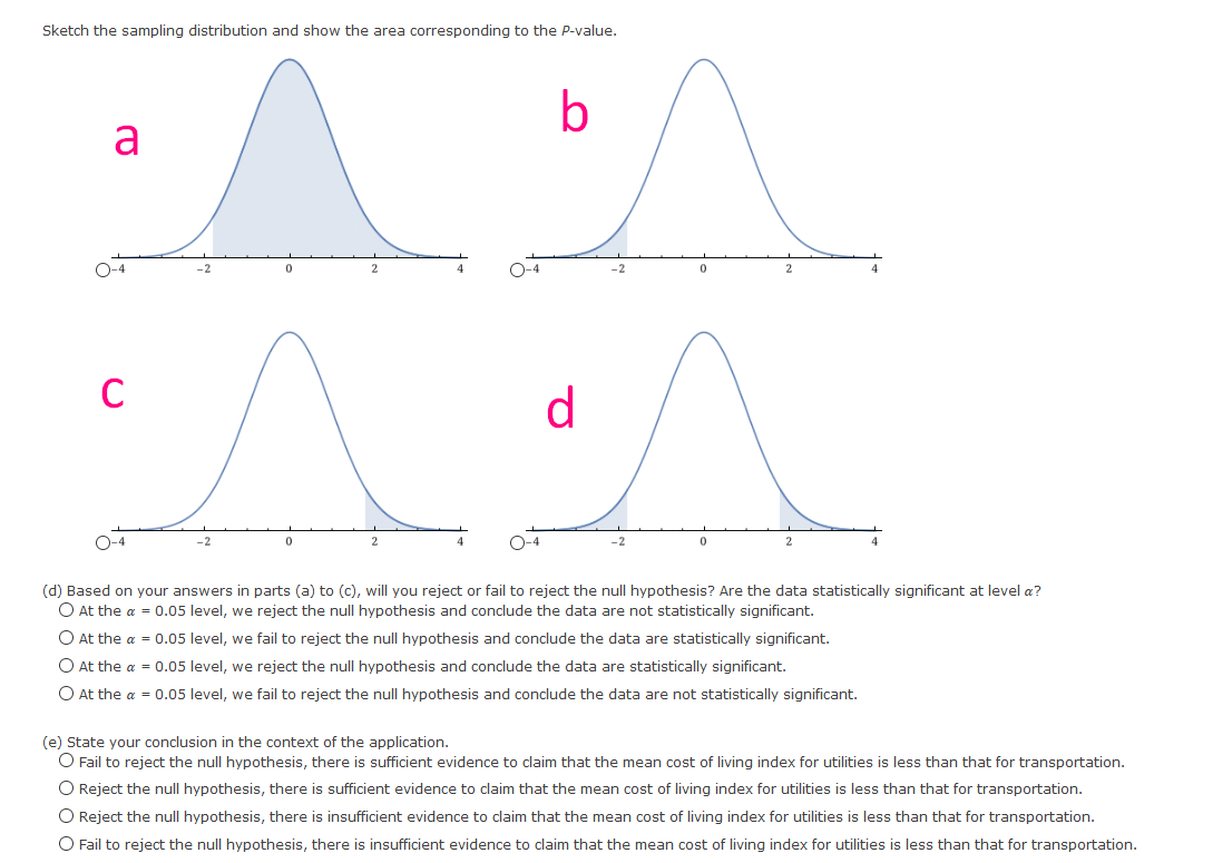
Transcribed Image Text:Sketch the sampling distribution and show the area corresponding to the P-value.
b
a
O-4
O-4
-2
C
d
O-4
O-4
(d) Based on your answers in parts (a) to (c), will you reject or fail to reject the null hypothesis? Are the data statistically significant at level a?
O At the a = 0.05 level, we reject the null hypothesis and conclude the data are not statistically significant.
O At the a = 0.05 level, we fail to reject the null hypothesis and conclude the data are statistically significant.
O At the a = 0.05 level, we reject the null hypothesis and conclude the data are statistically significant.
O At the a = 0.05 level, we fail to reject the null hypothesis and conclude the data are not statistically significant.
(e) State your conclusion in the context of the application.
O Fail to reject the null hypothesis, there is sufficient evidence to claim that the mean cost of living index for utilities is less than that for transportation.
O Reject the null hypothesis, there is sufficient evidence to claim that the mean cost of living index for utilities is less than that for transportation.
O Reject the null hypothesis, there is insufficient evidence to claim that the mean cost of living index for utilities is less than that for transportation.
O Fail to reject the null hypothesis, there is insufficient evidence to claim that the mean cost of living index for utilities is less than that for transportation.
Expert Solution
This question has been solved!
Explore an expertly crafted, step-by-step solution for a thorough understanding of key concepts.

Step by step
Solved in 2 steps with 1 images

Knowledge Booster


Learn more about
Need a deep-dive on the concept behind this application? Look no further. Learn more about this topic, statistics and related others by exploring similar questions and additional content below.Recommended textbooks for you
Glencoe Algebra 1, Student Edition, 9780079039897…
Algebra
ISBN:
9780079039897
Author:
Carter
Publisher:
McGraw Hill
Glencoe Algebra 1, Student Edition, 9780079039897…
Algebra
ISBN:
9780079039897
Author:
Carter
Publisher:
McGraw Hill