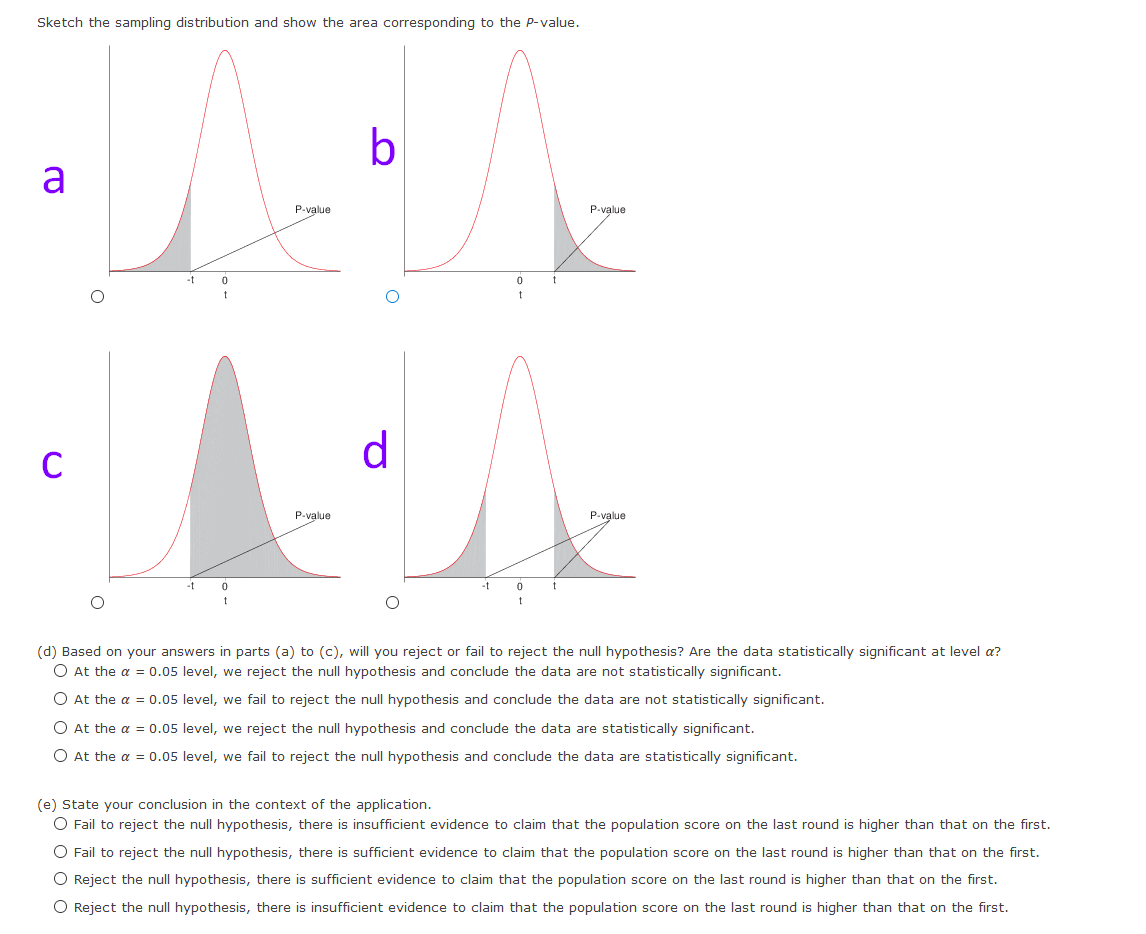
Sketch the sampling distribution and show the area corresponding to the P-value. b a P-value P-value -t d. P-value P-value -t -t (d) Based on your answers in parts (a) to (c), will you reject or fail to reject the null hypothesis? Are the data statistically significant at level a? O At the a = 0.05 level, we reject the null hypothesis and conclude the data are not statistically significant. O At the a = 0.05 level, we fail to reject the null hypothesis and conclude the data are not statistically significant. O At the a = 0.05 level, we reject the null hypothesis and conclude the data are statistically significant. O At the a = 0.05 level, we fail to reject the null hypothesis and conclude the data are statistically significant. (e) State your conclusion in the context of the application. O Fail to reject the null hypothesis, there is insufficient evidence to claim that the population score on the last round is higher than that on the first O Fail to reject the null hypothesis, there is sufficient evidence to claim that the population score on the last round is higher than that on the first. O Reject the null hypothesis, there is sufficient evidence to claim that the population score on the last round is higher than that on the first. O Reject the null hypothesis, there is insufficient evidence to claim that the population score on the last round is higher than that on the first.


In this problem, assume that the distribution of differences is approximately normal. Note: For degrees of freedom d.f. not in the Student's t table, use the closest d.f. that is smaller. In some situations, this choice of d.f. may increase the P-value by a small amount and therefore produce a slightly more "conservative" answer.
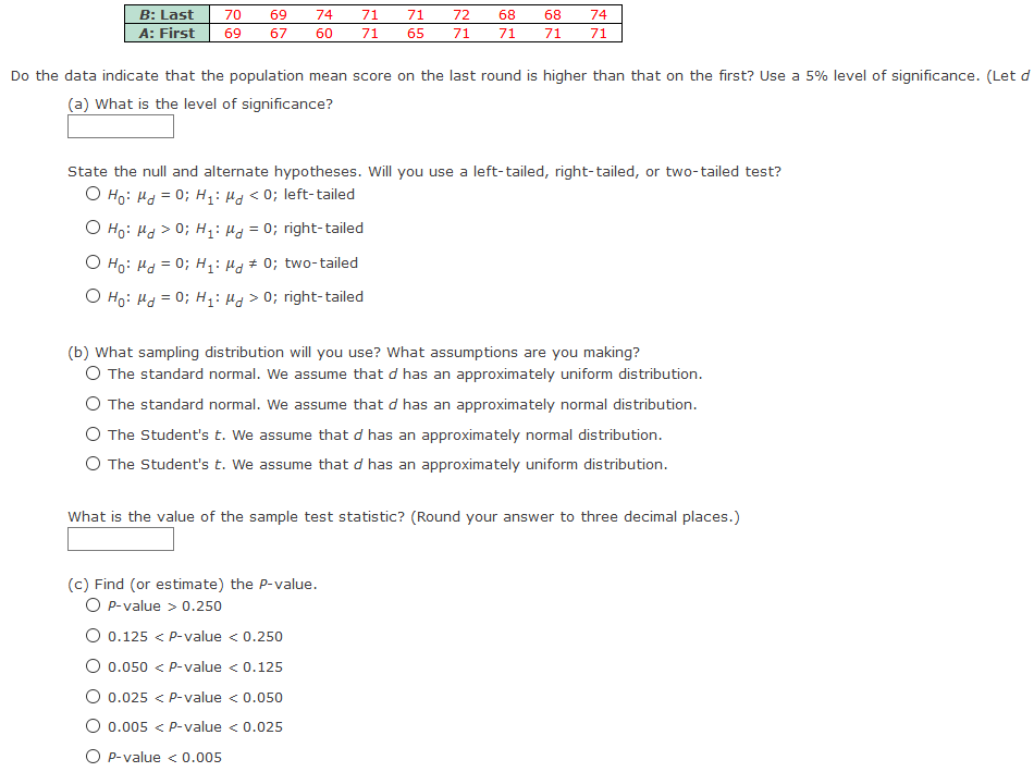
Do professional golfers play better in their last round? Let row B represent the score in the fourth (and final) round, and let row A represent the score in the first round of a professional golf tournament. A random sample of finalists in the British Open gave the following data for their first and last rounds in the tournament.
I need help with (c), sketching the distribution, (d) and (e)


Trending now
This is a popular solution!

Step by step
Solved in 6 steps


