> Income <- c(4016, 3159, 5100, 4742, 1864, 4070, 2731, 3348, 4764, 5573, 2583, 3866, 3586, 5037, 3605, 5345, 5370$ >Credit <-c(4016, 3159, 5100, 4742, 1864, 4070, 2731, 3348, 4764, 5573, 2583, 3866, 3586, 5037, 3605, 5345, 5370$ > Size <- c(3, 2, 4, 5, 2, 2, 1, 2, 4, 6, 1, 2, 5, 4, 2, 5, 6, 2, 3, 3, 4, 1, 2, 3, 4, 6, 2, 1, 5, 6, 3, 6, 2, 5, $ > Income <- c(54, 30, 32, 50, 31, 55, 37, 40, 66, 54, 30, 48, 34, 67, 50, 67, 55, 52, 51, 25, 48, 27, 33, 65, 63, $ > model <- 1m (Credit Income + Size) > summary (model) Call: 1m (formula Credit Income + Size) Residuals: Min 1Q Median 3Q Max 1270.10 -1172.67 -169.44 15.63 161.81 Coefficients: Estimate Std. Errort value Pr (>1t|) (Intercept) 1257.003 197.279 6.372 7.35e-08 Income 3.929 8.369 7.20e-11*** 34.894 10.895 1.87e-14 *** 32.881 380.176 Size Signif. codes: 0.***** 0.001 *** 0.01 0.05 0.11 Residual standard error: 393.8 on 47 degrees of freedom Multiple R-squared: 0.8293, Adjusted R-squared: 0.822 F-statistic: 114.2 on 2 and 47 DF, p-value: < 2.2e-16 a) From the output, observe that the regression equation as follows: y=1257.003+32.881x Income +380.176x Size b) b) From the output, observe that the adjusted coefficient of determination value is 0.5945 This value indicates that how the model is likely to be useful in predicting the annual credit card changes. The model is most likely to be useful, because this value is high value. c) The null and alternative hypotheses as follows: Null hypotheses, Ho: the overall regression model is not significant. Alternative hypotheses, H: the overall regression model is significant. From the output, observe that F statistic is 114.2 The p value is approximately 0.0000 The level of significance is, α = 0.01 Compare the p value with the level of significa Here, the p value is less than the level of significance, so reject the Null hypotheses. Hence, conclude that the overall regression model is significant. d) The Null and Alternative hypotheses for income coefficient as follows: Null hypotheses, Ho: B₁=0 Alternative hypotheses, H: B₁ #0 a From the output, observe that the test statistic value for income coefficient is 8.369 The p value is 0.0000 The level of significance is, α = 0.01 Compare the p value with the level of significance. Here, the p value is less than the level of significance, so reject the Null hypotheses. Hence, conclude that the slope coefficient for income variable is significant. The Null and Alternative hypotheses for Size coefficient as follows: Null hypotheses, H: ₂ = 0 Alternative hypotheses, H: B₂ #0 From the output, observe that the test statistic value for income coefficient is 10.895 The p value is 0.0000 The level of significance is, α = 0.01 Compare the p value with the level of significance. Here, the p value is less than the level of significance, so reject the Null hypotheses. Hence, conclude that the slope coefficient for size variable is significant. e) If increasing every one household in size, then the annual credit card charge will also be increases by 380.176 dollars when the income variable is treated as constant. If increasing every one dollar in income, then the annual credit card charge will also increases by 32.881 dollars when size variable is treated as constant. Yes. There is some logical interpretation in this time for y intercept, because the average annual credit card charges is not 1257.003 when size and income variables are treated as constants. This is not logical for this model. I
> Income <- c(4016, 3159, 5100, 4742, 1864, 4070, 2731, 3348, 4764, 5573, 2583, 3866, 3586, 5037, 3605, 5345, 5370$ >Credit <-c(4016, 3159, 5100, 4742, 1864, 4070, 2731, 3348, 4764, 5573, 2583, 3866, 3586, 5037, 3605, 5345, 5370$ > Size <- c(3, 2, 4, 5, 2, 2, 1, 2, 4, 6, 1, 2, 5, 4, 2, 5, 6, 2, 3, 3, 4, 1, 2, 3, 4, 6, 2, 1, 5, 6, 3, 6, 2, 5, $ > Income <- c(54, 30, 32, 50, 31, 55, 37, 40, 66, 54, 30, 48, 34, 67, 50, 67, 55, 52, 51, 25, 48, 27, 33, 65, 63, $ > model <- 1m (Credit Income + Size) > summary (model) Call: 1m (formula Credit Income + Size) Residuals: Min 1Q Median 3Q Max 1270.10 -1172.67 -169.44 15.63 161.81 Coefficients: Estimate Std. Errort value Pr (>1t|) (Intercept) 1257.003 197.279 6.372 7.35e-08 Income 3.929 8.369 7.20e-11*** 34.894 10.895 1.87e-14 *** 32.881 380.176 Size Signif. codes: 0.***** 0.001 *** 0.01 0.05 0.11 Residual standard error: 393.8 on 47 degrees of freedom Multiple R-squared: 0.8293, Adjusted R-squared: 0.822 F-statistic: 114.2 on 2 and 47 DF, p-value: < 2.2e-16 a) From the output, observe that the regression equation as follows: y=1257.003+32.881x Income +380.176x Size b) b) From the output, observe that the adjusted coefficient of determination value is 0.5945 This value indicates that how the model is likely to be useful in predicting the annual credit card changes. The model is most likely to be useful, because this value is high value. c) The null and alternative hypotheses as follows: Null hypotheses, Ho: the overall regression model is not significant. Alternative hypotheses, H: the overall regression model is significant. From the output, observe that F statistic is 114.2 The p value is approximately 0.0000 The level of significance is, α = 0.01 Compare the p value with the level of significa Here, the p value is less than the level of significance, so reject the Null hypotheses. Hence, conclude that the overall regression model is significant. d) The Null and Alternative hypotheses for income coefficient as follows: Null hypotheses, Ho: B₁=0 Alternative hypotheses, H: B₁ #0 a From the output, observe that the test statistic value for income coefficient is 8.369 The p value is 0.0000 The level of significance is, α = 0.01 Compare the p value with the level of significance. Here, the p value is less than the level of significance, so reject the Null hypotheses. Hence, conclude that the slope coefficient for income variable is significant. The Null and Alternative hypotheses for Size coefficient as follows: Null hypotheses, H: ₂ = 0 Alternative hypotheses, H: B₂ #0 From the output, observe that the test statistic value for income coefficient is 10.895 The p value is 0.0000 The level of significance is, α = 0.01 Compare the p value with the level of significance. Here, the p value is less than the level of significance, so reject the Null hypotheses. Hence, conclude that the slope coefficient for size variable is significant. e) If increasing every one household in size, then the annual credit card charge will also be increases by 380.176 dollars when the income variable is treated as constant. If increasing every one dollar in income, then the annual credit card charge will also increases by 32.881 dollars when size variable is treated as constant. Yes. There is some logical interpretation in this time for y intercept, because the average annual credit card charges is not 1257.003 when size and income variables are treated as constants. This is not logical for this model. I

Algebra: Structure And Method, Book 1
(REV)00th Edition
ISBN:9780395977224
Author:Richard G. Brown, Mary P. Dolciani, Robert H. Sorgenfrey, William L. Cole
Publisher:Richard G. Brown, Mary P. Dolciani, Robert H. Sorgenfrey, William L. Cole
Chapter2: Working With Real Numbers
Section2.3: Rules For Addition
Problem 9P

Related questions
Question
Transcribed Image Text:> Income <- c(4016, 3159, 5100, 4742, 1864, 4070, 2731, 3348, 4764, 5573, 2583, 3866, 3586, 5037, 3605, 5345, 5370$
>Credit <-c(4016, 3159, 5100, 4742, 1864, 4070, 2731, 3348, 4764, 5573, 2583, 3866, 3586, 5037, 3605, 5345, 5370$
> Size <- c(3, 2, 4, 5, 2, 2, 1, 2, 4, 6, 1, 2, 5, 4, 2, 5, 6, 2, 3, 3, 4, 1, 2, 3, 4, 6, 2, 1, 5, 6, 3, 6, 2, 5, $
> Income <- c(54, 30, 32, 50, 31, 55, 37, 40, 66, 54, 30, 48, 34, 67, 50, 67, 55, 52, 51, 25, 48, 27, 33, 65, 63, $
> model <- 1m (Credit Income + Size)
> summary (model)
Call:
1m (formula Credit Income + Size)
Residuals:
Min
1Q
Median
3Q
Max
1270.10
-1172.67 -169.44
15.63 161.81
Coefficients:
Estimate Std. Errort value Pr (>1t|)
(Intercept) 1257.003 197.279 6.372 7.35e-08
Income
3.929 8.369 7.20e-11***
34.894 10.895 1.87e-14 ***
32.881
380.176
Size
Signif. codes: 0.***** 0.001 *** 0.01 0.05 0.11
Residual standard error: 393.8 on 47 degrees of freedom
Multiple R-squared: 0.8293,
Adjusted R-squared: 0.822
F-statistic: 114.2 on 2 and 47 DF, p-value: < 2.2e-16
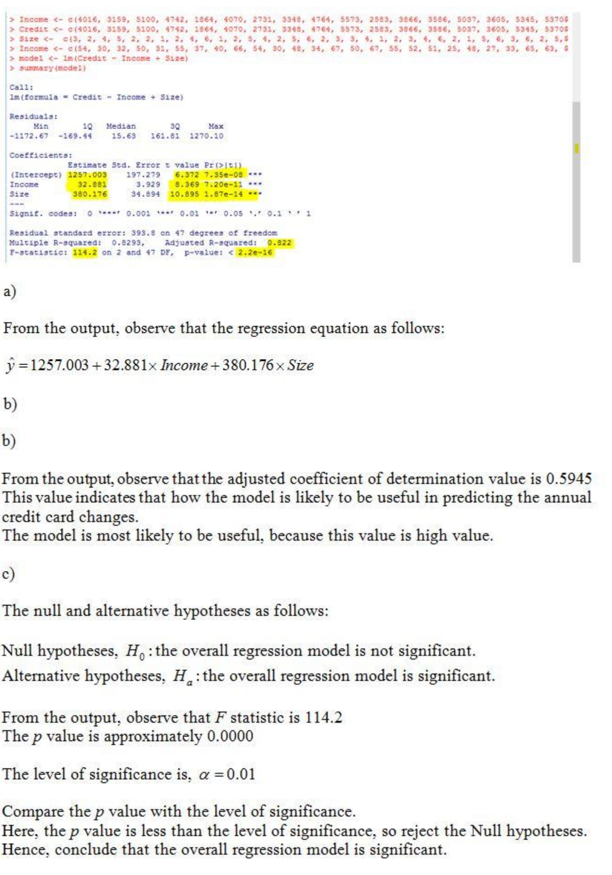
a)
From the output, observe that the regression equation as follows:
y=1257.003+32.881x Income +380.176x Size
b)
b)
From the output, observe that the adjusted coefficient of determination value is 0.5945
This value indicates that how the model is likely to be useful in predicting the annual
credit card changes.
The model is most likely to be useful, because this value is high value.
c)
The null and alternative hypotheses as follows:
Null hypotheses, Ho: the overall regression model is not significant.
Alternative hypotheses, H: the overall regression model is significant.
From the output, observe that F statistic is 114.2
The p value is approximately 0.0000
The level of significance is, α = 0.01
Compare the p value with the level of significa
Here, the p value is less than the level of significance, so reject the Null hypotheses.
Hence, conclude that the overall regression model is significant.
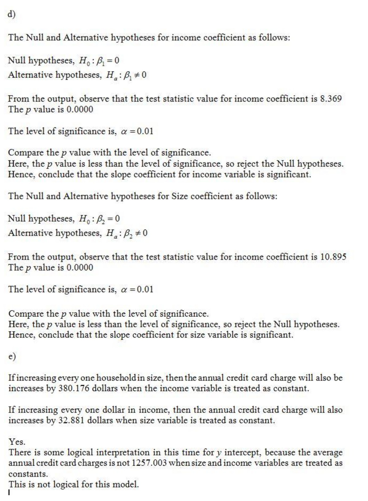
Transcribed Image Text:d)
The Null and Alternative hypotheses for income coefficient as follows:
Null hypotheses, Ho: B₁=0
Alternative hypotheses, H: B₁ #0
a
From the output, observe that the test statistic value for income coefficient is 8.369
The p value is 0.0000
The level of significance is, α = 0.01
Compare the p value with the level of significance.
Here, the p value is less than the level of significance, so reject the Null hypotheses.
Hence, conclude that the slope coefficient for income variable is significant.
The Null and Alternative hypotheses for Size coefficient as follows:
Null hypotheses, H: ₂ = 0
Alternative hypotheses, H: B₂ #0
From the output, observe that the test statistic value for income coefficient is 10.895
The p value is 0.0000
The level of significance is, α = 0.01
Compare the p value with the level of significance.
Here, the p value is less than the level of significance, so reject the Null hypotheses.
Hence, conclude that the slope coefficient for size variable is significant.
e)
If increasing every one household in size, then the annual credit card charge will also be
increases by 380.176 dollars when the income variable is treated as constant.
If increasing every one dollar in income, then the annual credit card charge will also
increases by 32.881 dollars when size variable is treated as constant.
Yes.
There is some logical interpretation in this time for y intercept, because the average
annual credit card charges is not 1257.003 when size and income variables are treated as
constants.
This is not logical for this model.
I
Expert Solution
This question has been solved!
Explore an expertly crafted, step-by-step solution for a thorough understanding of key concepts.

Step by step
Solved in 2 steps with 1 images

Recommended textbooks for you
Algebra: Structure And Method, Book 1
Algebra
ISBN:
9780395977224
Author:
Richard G. Brown, Mary P. Dolciani, Robert H. Sorgenfrey, William L. Cole
Publisher:
McDougal Littell

Intermediate Algebra
Algebra
ISBN:
9781285195728
Author:
Jerome E. Kaufmann, Karen L. Schwitters
Publisher:
Cengage Learning

Algebra for College Students
Algebra
ISBN:
9781285195780
Author:
Jerome E. Kaufmann, Karen L. Schwitters
Publisher:
Cengage Learning
Algebra: Structure And Method, Book 1
Algebra
ISBN:
9780395977224
Author:
Richard G. Brown, Mary P. Dolciani, Robert H. Sorgenfrey, William L. Cole
Publisher:
McDougal Littell
Intermediate Algebra
Algebra
ISBN:
9781285195728
Author:
Jerome E. Kaufmann, Karen L. Schwitters
Publisher:
Cengage Learning
Algebra for College Students
Algebra
ISBN:
9781285195780
Author:
Jerome E. Kaufmann, Karen L. Schwitters
Publisher:
Cengage Learning