the ed. 11.2 General Concepts 459 TABLE 11.1 Sample data from the Greene-Touchstone study relating birthweight and estriol level in pregnant women near term Estriol Birthweight (mg/24 hr) (g/100) Estriol (mg/24 hr) Birthweight (g/100) X; Y₁ Xi Yi 2 12 7 25 17 17 32 9 25 18 25 32 3 9 25 19 27 34 4 12 27 20 15 34 5 14 27 21 15 34 6 16 27 22 15 35 7 16 24 23 16 35 8 14 30 24 19 34 9 16 30 25 18 35 10 16 31 26 17 36 11 17 30 27 18 37 12 19 31 28 20 38 13 21 30 29 22 40 14 24 28 30 25 39 15 15 32 31 24 43 16 16 32 EQUATION 11.2 DEFINITION 11.2 EXAMPLE 11.4 EXAMPLE 11.5 Source: Based on the American Journal of Obstetrics and Gynecology, 85(1), 1-9, 1963. Let's assume e follows a normal distribution, with mean 0 and variance o². The full linear-regression model then takes the following form: y = a+ẞx+e where e is normally distributed with mean 0 and variance σ². For any linear-regression equation of the form y=a+ẞx+e, y is called the depen- dent variable and x is called the independent variable because we are trying to predict y as a function of x. Obstetrics Birthweight is the dependent variable and estriol is the independent variable for the problem posed in Example 11.3 because estriol levels are being used to try to predict birthweight. One interpretation of the regression line is that for a woman with estriol level x, the corresponding birthweight will be normally distributed with mean a + ẞx and variance o². If σ2 were 0, then every point would fall exactly on the regression line, whereas the larger o² is, the more scatter occurs about the regression line. This rela- tionship is illustrated in Figure 11.2. How can ẞ be interpreted? If ẞ is greater than 0, then as x increases, the expected value of y = a + ẞx will increase. Obstetrics This situation appears to be the case in Figure 11.3a for birthweight (y) and estriol (x) because as estriol increases, the average birthweight correspondingly increases. If ẞ is less than 0, then as x increases, the expected value of y will decrease.
the ed. 11.2 General Concepts 459 TABLE 11.1 Sample data from the Greene-Touchstone study relating birthweight and estriol level in pregnant women near term Estriol Birthweight (mg/24 hr) (g/100) Estriol (mg/24 hr) Birthweight (g/100) X; Y₁ Xi Yi 2 12 7 25 17 17 32 9 25 18 25 32 3 9 25 19 27 34 4 12 27 20 15 34 5 14 27 21 15 34 6 16 27 22 15 35 7 16 24 23 16 35 8 14 30 24 19 34 9 16 30 25 18 35 10 16 31 26 17 36 11 17 30 27 18 37 12 19 31 28 20 38 13 21 30 29 22 40 14 24 28 30 25 39 15 15 32 31 24 43 16 16 32 EQUATION 11.2 DEFINITION 11.2 EXAMPLE 11.4 EXAMPLE 11.5 Source: Based on the American Journal of Obstetrics and Gynecology, 85(1), 1-9, 1963. Let's assume e follows a normal distribution, with mean 0 and variance o². The full linear-regression model then takes the following form: y = a+ẞx+e where e is normally distributed with mean 0 and variance σ². For any linear-regression equation of the form y=a+ẞx+e, y is called the depen- dent variable and x is called the independent variable because we are trying to predict y as a function of x. Obstetrics Birthweight is the dependent variable and estriol is the independent variable for the problem posed in Example 11.3 because estriol levels are being used to try to predict birthweight. One interpretation of the regression line is that for a woman with estriol level x, the corresponding birthweight will be normally distributed with mean a + ẞx and variance o². If σ2 were 0, then every point would fall exactly on the regression line, whereas the larger o² is, the more scatter occurs about the regression line. This rela- tionship is illustrated in Figure 11.2. How can ẞ be interpreted? If ẞ is greater than 0, then as x increases, the expected value of y = a + ẞx will increase. Obstetrics This situation appears to be the case in Figure 11.3a for birthweight (y) and estriol (x) because as estriol increases, the average birthweight correspondingly increases. If ẞ is less than 0, then as x increases, the expected value of y will decrease.

Linear Algebra: A Modern Introduction
4th Edition
ISBN:9781285463247
Author:David Poole
Publisher:David Poole
Chapter7: Distance And Approximation
Section7.3: Least Squares Approximation
Problem 31EQ

Related questions
Question
Example 11.1 Please solve using R. Obstetricians sometimes order tests for es-
triol levels from 24-hour urine specimens taken from preg-
nant women who are near term, because level of estriol has
been found to be related to infant birthweight. The test
can provide indirect evidence of an abnormally small fetus.
The relationship between estriol level and birthweight can
be quantified by fitting a regression line that relates the
two variables. Data is given in Table 11.1 on page 459.
Transcribed Image Text:the
ed.
11.2
General Concepts
459
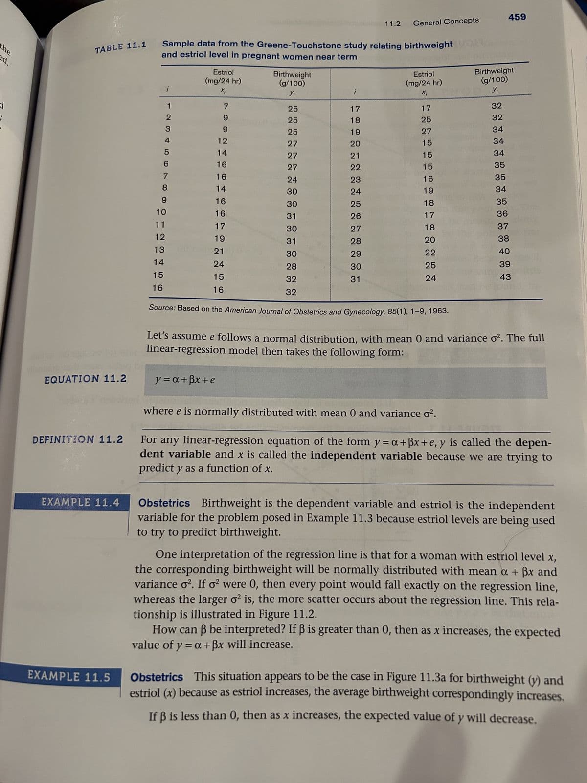
TABLE 11.1
Sample data from the Greene-Touchstone study relating birthweight
and estriol level in pregnant women near term
Estriol
Birthweight
(mg/24 hr)
(g/100)
Estriol
(mg/24 hr)
Birthweight
(g/100)
X;
Y₁
Xi
Yi
2
12
7
25
17
17
32
9
25
18
25
32
3
9
25
19
27
34
4
12
27
20
15
34
5
14
27
21
15
34
6
16
27
22
15
35
7
16
24
23
16
35
8
14
30
24
19
34
9
16
30
25
18
35
10
16
31
26
17
36
11
17
30
27
18
37
12
19
31
28
20
38
13
21
30
29
22
40
14
24
28
30
25
39
15
15
32
31
24
43
16
16
32
EQUATION 11.2
DEFINITION 11.2
EXAMPLE 11.4
EXAMPLE 11.5
Source: Based on the American Journal of Obstetrics and Gynecology, 85(1), 1-9, 1963.
Let's assume e follows a normal distribution, with mean 0 and variance o². The full
linear-regression model then takes the following form:
y = a+ẞx+e
where e is normally distributed with mean 0 and variance σ².
For any linear-regression equation of the form y=a+ẞx+e, y is called the depen-
dent variable and x is called the independent variable because we are trying to
predict y as a function of x.
Obstetrics Birthweight is the dependent variable and estriol is the independent
variable for the problem posed in Example 11.3 because estriol levels are being used
to try to predict birthweight.
One interpretation of the regression line is that for a woman with estriol level x,
the corresponding birthweight will be normally distributed with mean a + ẞx and
variance o². If σ2 were 0, then every point would fall exactly on the regression line,
whereas the larger o² is, the more scatter occurs about the regression line. This rela-
tionship is illustrated in Figure 11.2.
How can ẞ be interpreted? If ẞ is greater than 0, then as x increases, the expected
value of y = a + ẞx will increase.
Obstetrics This situation appears to be the case in Figure 11.3a for birthweight (y) and
estriol (x) because as estriol increases, the average birthweight correspondingly increases.
If ẞ is less than 0, then as x increases, the expected value of y will decrease.
Expert Solution
This question has been solved!
Explore an expertly crafted, step-by-step solution for a thorough understanding of key concepts.

Step by step
Solved in 2 steps with 1 images

Recommended textbooks for you
Linear Algebra: A Modern Introduction
Algebra
ISBN:
9781285463247
Author:
David Poole
Publisher:
Cengage Learning

Functions and Change: A Modeling Approach to Coll…
Algebra
ISBN:
9781337111348
Author:
Bruce Crauder, Benny Evans, Alan Noell
Publisher:
Cengage Learning

Glencoe Algebra 1, Student Edition, 9780079039897…
Algebra
ISBN:
9780079039897
Author:
Carter
Publisher:
McGraw Hill
Linear Algebra: A Modern Introduction
Algebra
ISBN:
9781285463247
Author:
David Poole
Publisher:
Cengage Learning
Functions and Change: A Modeling Approach to Coll…
Algebra
ISBN:
9781337111348
Author:
Bruce Crauder, Benny Evans, Alan Noell
Publisher:
Cengage Learning
Glencoe Algebra 1, Student Edition, 9780079039897…
Algebra
ISBN:
9780079039897
Author:
Carter
Publisher:
McGraw Hill

Trigonometry (MindTap Course List)
Trigonometry
ISBN:
9781337278461
Author:
Ron Larson
Publisher:
Cengage Learning