The propensity to consume tells us by how much consumption changes for a given change in disposable income. To analyze this fact, follow these steps: 5- Go to the Federal Reserve Economic Data (FRED) https://fred.stlouisfed.org/. download the series A067RX1A020NBEA and PCECCA since 1999. Make sure all series are in real terms and in comparable units. Compile a single spreadsheet with these series. 6- In the spreadsheet, first compute the annual growth rate of disposable income and consumption for all years in the sample. Then compute the average for the period 2000-2017 for both variables. Finally, construct a demeaned measure of the annual growth rate of disposable income and consumption for all years in the sample. That is, let C t denote consumption in year t. Then, the growth rate of consumption between year t and t−1 is [(C t /C t−1 )−1], denoted by gC t. Now, let gC denote the average annual growth rate in consumption since 2000 . This number will stay fixed and not changing over time. Then the demeaned measure of the annual growth rate of consumption is gC t − gC for year t. (See Appendix 3 for more information). 7- Include a scatter plot of the demeaned measure of the annual growth rate of consumption and the demeaned measure of disposable income for the period 2000-2017. Use the x-axis for the demeaned growth rate of disposable income and the y-axis for the demeaned growth rate of consumption. Include axis titles for both variables. 8- Finally, add a linear trend line of the scatter plot and show the equation. 9- The equation that Excel produces for the trend line will have the following form: y=bx+e, where y is the growth rate of consumption, x is the growth rate of disposable income, b is a coefficient, and e will be close to zero. 10- Find b, the propensity to consume. Discuss how an increase in disposable income of $1 billion above the average is typically associated with an increase in consumption of $ b billion above the average.
The propensity to consume tells us by how much consumption changes for a given change in disposable income. To analyze this fact, follow these steps: 5- Go to the Federal Reserve Economic Data (FRED) https://fred.stlouisfed.org/. download the series A067RX1A020NBEA and PCECCA since 1999. Make sure all series are in real terms and in comparable units. Compile a single spreadsheet with these series. 6- In the spreadsheet, first compute the annual growth rate of disposable income and consumption for all years in the sample. Then compute the average for the period 2000-2017 for both variables. Finally, construct a demeaned measure of the annual growth rate of disposable income and consumption for all years in the sample. That is, let C t denote consumption in year t. Then, the growth rate of consumption between year t and t−1 is [(C t /C t−1 )−1], denoted by gC t. Now, let gC denote the average annual growth rate in consumption since 2000 . This number will stay fixed and not changing over time. Then the demeaned measure of the annual growth rate of consumption is gC t − gC for year t. (See Appendix 3 for more information). 7- Include a scatter plot of the demeaned measure of the annual growth rate of consumption and the demeaned measure of disposable income for the period 2000-2017. Use the x-axis for the demeaned growth rate of disposable income and the y-axis for the demeaned growth rate of consumption. Include axis titles for both variables. 8- Finally, add a linear trend line of the scatter plot and show the equation. 9- The equation that Excel produces for the trend line will have the following form: y=bx+e, where y is the growth rate of consumption, x is the growth rate of disposable income, b is a coefficient, and e will be close to zero. 10- Find b, the propensity to consume. Discuss how an increase in disposable income of $1 billion above the average is typically associated with an increase in consumption of $ b billion above the average.

Chapter9: Aggregate Demand
Section: Chapter Questions
Problem 1.1P

Related questions
Question
The propensity to consume tells us by how much consumption changes for a given change in disposable income. To analyze this fact, follow these steps: 5- Go to the Federal Reserve Economic Data (FRED) https://fred.stlouisfed.org/. download the series A067RX1A020NBEA and PCECCA since 1999. Make sure all series are in real terms and in comparable units. Compile a single spreadsheet with these series. 6- In the spreadsheet, first compute the annual growth rate of disposable income and consumption for all years in the sample. Then compute the average for the period 2000-2017 for both variables. Finally, construct a demeaned measure of the annual growth rate of disposable income and consumption for all years in the sample. That is, let C
t denote consumption in year t. Then, the growth rate of consumption between year t and t−1 is [(C t /C t−1 )−1], denoted by gC t. Now, let gC denote the average annual growth rate in consumption since 2000 . This number will stay fixed and not changing over time. Then the demeaned measure of the annual growth rate of consumption is gC t − gC for year t. (See Appendix 3 for more information). 7- Include a scatter plot of the demeaned measure of the annual growth rate of consumption and the demeaned measure of disposable income for the period 2000-2017. Use the x-axis for the demeaned growth rate of disposable income and the y-axis for the demeaned growth rate of consumption. Include axis titles for both variables. 8- Finally, add a linear trend line of the scatter plot and show the equation. 9- The equation that Excel produces for the trend line will have the following form: y=bx+e, where y is the growth rate of consumption, x is the growth rate of disposable income, b is a coefficient, and e will be close to zero. 10- Find b, the propensity to consume. Discuss how an increase in disposable income of $1 billion above the average is typically associated with an increase in consumption of $ b billion above the average.
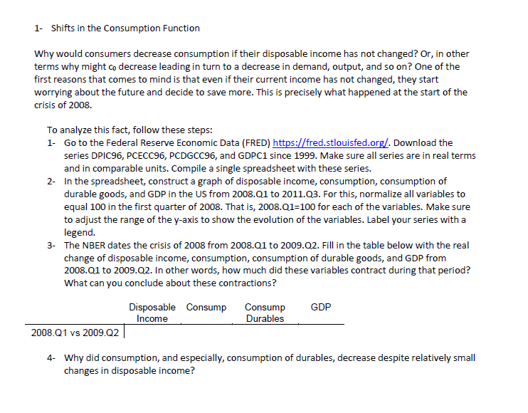
Transcribed Image Text:1- Shifts in the Consumption Function
Why would consumers decrease consumption if their disposable income has not changed? Or, in other
terms why might co decrease leading in turn to a decrease in demand, output, and so on? One of the
first reasons that comes to mind is that even if their current income has not changed, they start
worrying about the future and decide to save more. This is precisely what happened at the start of the
crisis of 2008.
To analyze this fact, follow these steps:
1-
Go to the Federal Reserve Economic Data (FRED) https://fred.stlouisfed.org/. Download the
series DPIC96, PCECC96, PCDGCC96, and GDPC1 since 1999. Make sure all series are in real terms
and in comparable units. Compile a single spreadsheet with these series.
2- In the spreadsheet, construct a graph of disposable income, consumption, consumption of
durable goods, and GDP in the US from 2008.Q1 to 2011.Q3. For this, normalize all variables to
equal 100 in the first quarter of 2008. That is, 2008.Q1=100 for each of the variables. Make sure
to adjust the range of the y-axis to show the evolution of the variables. Label your series with a
legend.
3- The NBER dates the crisis of 2008 from 2008.Q1 to 2009.Q2. Fill in the table below with the real
change of disposable income, consumption, consumption of durable goods, and GDP from
2008.Q1 to 2009.Q2. In other words, how much did these variables contract during that period?
What can you conclude about these contractions?
Disposable Consump
Income
Consump
Durables
GDP
2008.Q1 vs 2009.Q2
4- Why did consumption, and especially, consumption of durables, decrease despite relatively small
changes in disposable income?
Expert Solution
This question has been solved!
Explore an expertly crafted, step-by-step solution for a thorough understanding of key concepts.

This is a popular solution!

Trending now
This is a popular solution!

Step by step
Solved in 6 steps with 1 images

Knowledge Booster


Learn more about
Need a deep-dive on the concept behind this application? Look no further. Learn more about this topic, economics and related others by exploring similar questions and additional content below.Recommended textbooks for you

Macroeconomics: Principles and Policy (MindTap Co…
Economics
ISBN:
9781305280601
Author:
William J. Baumol, Alan S. Blinder
Publisher:
Cengage Learning

Essentials of Economics (MindTap Course List)
Economics
ISBN:
9781337091992
Author:
N. Gregory Mankiw
Publisher:
Cengage Learning
Macroeconomics: Principles and Policy (MindTap Co…
Economics
ISBN:
9781305280601
Author:
William J. Baumol, Alan S. Blinder
Publisher:
Cengage Learning
Essentials of Economics (MindTap Course List)
Economics
ISBN:
9781337091992
Author:
N. Gregory Mankiw
Publisher:
Cengage Learning

Brief Principles of Macroeconomics (MindTap Cours…
Economics
ISBN:
9781337091985
Author:
N. Gregory Mankiw
Publisher:
Cengage Learning

