You need to test whether the average mealtime spending of American tourists (population 1) is greater than that for British tourists (population 2). Assume that you have a sample of n1=7 with sample mean X1=40 and a sample standard deviation of S1=6, and you have an independent sample of n2=16 from another population with a sample mean of X2=31 and sample standard deviation S2=5. Complete parts (a) to (d). Click here to view page 1 of the table of the critical values of t. LOADING... Click here to view page 2 of the table of the critical values of t. LOADING... a. What is the value of the pooled-variance t test statistic for testing? t=enter your response here (Type an integer or a decimal rounded to two decimal places as needed.) b. In finding the critical value of the test statistic t, how many degrees of freedom are there? There are enter your response here degrees of freedom. c. Using a significance level of α=0.01, what is the critical value for a one-tail test of the hypothesis H0: μ1− μ2<0 against the alternative H1: μ1−μ2≥0? The critical value is enter your response here. (Type an integer or a decimal rounded to two decimal places as needed.) d. What is your statistical decision? A. Do not reject H0 because the calculated t test statistic is greater than the upper-tail critical value. B. Reject H0 because the calculated t test statistic is less than the upper-tail critical value. C. Reject H0 because the calculated t test statistic is greater than the upper-tail critical value. D. Do not reject H0 because the calculated t test statistic
You need to test whether the average mealtime spending of American tourists (population 1) is greater than that for British tourists (population 2). Assume that you have a sample of n1=7 with sample mean X1=40 and a sample standard deviation of S1=6, and you have an independent sample of n2=16 from another population with a sample mean of X2=31 and sample standard deviation S2=5. Complete parts (a) to (d). Click here to view page 1 of the table of the critical values of t. LOADING... Click here to view page 2 of the table of the critical values of t. LOADING... a. What is the value of the pooled-variance t test statistic for testing? t=enter your response here (Type an integer or a decimal rounded to two decimal places as needed.) b. In finding the critical value of the test statistic t, how many degrees of freedom are there? There are enter your response here degrees of freedom. c. Using a significance level of α=0.01, what is the critical value for a one-tail test of the hypothesis H0: μ1− μ2<0 against the alternative H1: μ1−μ2≥0? The critical value is enter your response here. (Type an integer or a decimal rounded to two decimal places as needed.) d. What is your statistical decision? A. Do not reject H0 because the calculated t test statistic is greater than the upper-tail critical value. B. Reject H0 because the calculated t test statistic is less than the upper-tail critical value. C. Reject H0 because the calculated t test statistic is greater than the upper-tail critical value. D. Do not reject H0 because the calculated t test statistic

MATLAB: An Introduction with Applications
6th Edition
ISBN:9781119256830
Author:Amos Gilat
Publisher:Amos Gilat
Chapter1: Starting With Matlab
Section: Chapter Questions
Problem 1P

Related questions
Question
You need to test whether the average mealtime spending of American tourists (population 1) is greater than that for British tourists (population 2). Assume that you have a sample of
n1=7
with sample mean
X1=40
and a sample standard deviation of
S1=6,
and you have an independent sample of
n2=16
from another population with a sample mean of
X2=31
and sample standard deviation
S2=5.
Complete parts (a) to (d).Click here to view page 1 of the table of the critical values of t.
LOADING...
Click here to view page 2 of the table of the critical values of t.
LOADING...
a. What is the value of the pooled-variance t test statistic for testing?
t=enter your response here
(Type an integer or a decimal rounded to two decimal places as needed.)
b. In finding the critical value of the test statistic t, how many degrees of freedom are there?
There are
enter your response here
degrees of freedom.c. Using a significance level of
α=0.01,
what is the critical value for a one-tail test of the hypothesis
H0: μ1− μ2<0
against the alternative
H1: μ1−μ2≥0?
The critical value is
enter your response here.
(Type an integer or a decimal rounded to two decimal places as needed.)
d. What is your statistical decision?
Do not reject
H0
because the calculated t test statistic is greater than the upper-tail critical value.Reject
H0
because the calculated t test statistic is less than the upper-tail critical value.Reject
H0
because the calculated t test statistic is greater than the upper-tail critical value.Do not reject
H0
because the calculated t test statistic is less than the upper-tail critical value.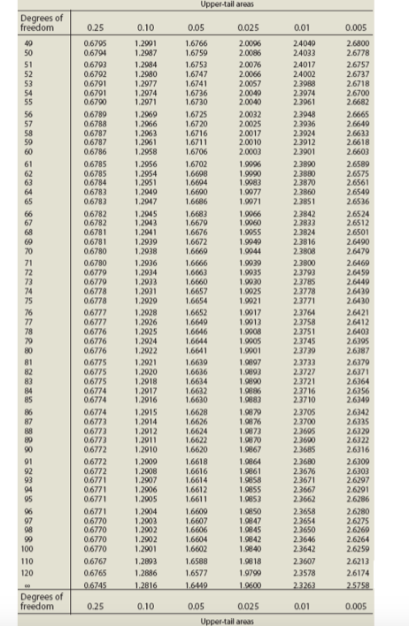
Transcribed Image Text:Upper-tail areas
Degrees of
freedom
0.25
0.10
0.05
0.025
0.01
0.005
40
50
0.6795
0.6794
1.2991
1.2987
1.6766
1.6759
2.0096
2.0086
2.4049
2.4033
2.6800
2.6778
51
52
0.6793
0.6792
0.6791
1.6753
1.6747
2.0076
2.0066
24017
24002
2.6757
2.6737
2.6718
1.2984
1.2980
1.2977
53
1.6741
2.0057
2.3988
54
55
0.6791
0.6790
1.2974
1.2971
1.6736
1.6730
2.0049
2.0040
2.3974
2.3961
2.6700
2.6682
0.6789
0.6788
0.6787
0.6787
1.2969
1.2966
1.2963
1.2961
2.3948
2.3936
2.3924
2.3912
2.6665
2.6649
2.6633
2.6618
2.6603
56
1.6725
2.0032
57
1.6720
1.6716
1.6711
2.0025
2.0017
2.0010
2.0003
60
0.6786
1.2958
1.6706
2.3901
61
0.6785
1.2956
1.6702
1.9996
2.3890
2.6589
1.2954
1.2951
1.2949
1.2947
1.9990
1.9983
1.9977
62
63
0.6785
0.6784
1.6698
1.6604
1.6600
2.3880
2.3870
2.3860
2.3851
2.6575
2.6561
2.6549
2.6536
0.6783
0.6783
64
65
1.6686
1.9971
66
67
0.6782
0.6782
1.2945
1.2943
1.2941
1.6683
1.6679
1.6676
1.9966
1.9060
1.9955
2.3842
2.3833
2.3824
2.6524
2.6512
68
0.6781
2.6501
69
0.6781
1.2939
1.6672
1.9949
2.3816
2.6490
70
0.6780
1.2938
1.6669
1.9944
2.3808
2.6479
1.2936
1.9939
2.6469
2.6459
2.6449
71
0.6780
0.6779
0.6779
1.6666
2.3800
72
73
1.6663
1.6660
1.6657
1.9935
1.9930
2.3793
2.3785
2.3778
2.3771
1.2934
1.2933
74
75
0.6778
0.6778
1.9025
1.2031
1.2929
2.6430
2.6430
1.6654
1.9921
76
77
78
79
0.6777
0.6777
0.6776
0.6776
2.3764
2.3758
2.3751
2.3745
2.3739
2.6421
2.6412
2.6403
2.6395
2.6387
1.2028
1.6652
1.9017
1.2926
1.2925
1.2924
1.6649
1.6646
1.6644
1.9913
1.9908
1.9005
80
0.6776
1.2922
1.6641
1.9001
0.6775
0.6775
2.3733
2.3727
2.3721
2.3716
2.3710
81
1.2921
1.6639
1.9897
1.9893
1.9890
1.9886
1.9883
2.6379
2.6371
1.2920
1.2918
1.2917
1.2916
82
1.6636
83
84
85
0.6775
0.6774
0.6774
1.6634
1.6632
1.6630
2.6364
2.6356
2.6349
0.6774
0.6773
0.6773
0.6773
86
87
1.2915
1.2914
1.6628
1.6626
1.6624
1.6622
1.9879
1.9876
1.0873
1.9870
2.3705
2.3700
2.6342
2.6335
2.6329
2.6322
88
89
1.2912
2.3605
2.3690
1.2011
90
0.6772
1.2910
1.6620
1.9867
2.3685
2.6316
91
92
93
0.6772
0.6772
0.6771
1.2909
1.2908
1.2907
1.2906
1.2905
1.6618
1.6616
1.6614
1.9864
1.9861
1.9858
1.9855
1.9853
2.3680
2.3676
2.3671
2.3667
2.3662
2.6300
2.6303
2.6297
94
0.6771
1.6612
2.6291
95
0.6771
1.6611
2.6286
2.6280
2.6275
2.6269
2.6264
2.6259
96
0.6771
1.2904
1.6609
1.6607
1.6606
1.6604
1.9850
1.9847
1.9845
1.9842
2.3658
97
98
99
0.6770
0.6770
0.6770
0.6770
1.2903
1.2902
1.2902
1.2901
2.3654
2.3650
2.3646
2.3642
100
1.6602
1.9840
1.9818
1.9799
110
0.6767
1.2893
1.6588
2.3607
2.6213
120
0.6765
1.2886
1.6577
2.3578
2.6174
0.6745
1.2816
1.6449
1.9600
2.3263
2.5758
Degrees of
freedom
0.25
0.10
0.05
0.025
0.01
0.005
Upper-tail areas
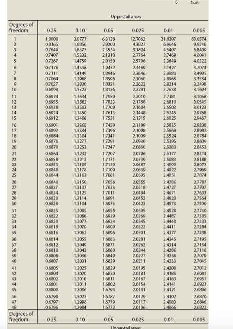
Transcribed Image Text:Upper-tail areas
Degrees of
freedom
0.25
0.10
0.05
0.025
0.01
0.005
1
1.0000
3.0777
6.3138
12.7062
31.8207
63.6574
2
3
1.8856
1.6377
1.5332
0.8165
2.9200
2.3534
4.3027
3.1824
6.9646
9.9248
5.8409
0.7649
4.5407
3.7469
0.7407
2.1318
2.7764
4.6041
07267
1.4759
2.0150
2.5706
3.3649
4.0322
07176
07111
1.4398
1.9432
2.4469
2.3646
2.3060
3.1427
3.7074
3.4995
3.3554
3.2408
1.4149
1.8946
2.9980
2.8065
2.8214
0.7064
1.3968
1.8595
0.7027
1.3830
1.8331
2.2622
2.2281
10
0.6998
1.3722
1.8125
2.7638
3.1693
0.6074
0.6955
0.6038
0.6924
3.1058
3.0545
3.0123
2.9768
11
1.3634
1.7959
2.2010
2.7181
1.7823
1.7709
1.7613
1.7531
12
1.3562
1.3502
1.3450
2.1788
2.1604
2.1448
2.1315
2.6810
13
14
2.6503
2.6245
15
0.6912
1.3406
2.6025
2.9467
16
0.6901
1.3368
1.7459
2.5835
2.1199
2.1098
2.9208
17
0.6892
1.3334
1.7396
2.5669
2.8982
18
19
0.6884
0.6876
1.7341
1.7291
2.1009
2.0030
2.5524
2.5395
1.3304
2.8784
2.8609
1.3277
20
0.6870
1.3253
1.7247
2.0860
2.5280
2.8453
1.3232
1.3212
1.3195
1.3178
21
0.6864
1.7207
2.0796
2.8314
2.0739
2.0687
2.0639
25177
2.5083
2.4999
2.4022
22
0.6858
1.7171
2.8188
23
24
25
1.7139
1.7109
2.8073
2.7969
2.7874
0.6853
0.6848
0.6844
1.3163
1.7081
2.0595
2.4851
26
0.6840
1.3150
1.7056
2.0555
2.0518
2.0484
2.0452
2.0423
2.4786
2.7787
27
28
29
30
0.6837
0.6834
0.6830
0.6828
1.3137
1.3125
1.3114
1.3104
1.7033
1.7011
1.6991
1.6973
2.4727
2.4671
2.4620
2.4573
2.7707
2.7633
2.7564
2.7500
31
0.6825
0.6822
1.3095
1.3086
1.3077
1.3070
1.3062
1.6955
2.0395
2.4528
2.7740
2.0360
2.0345
2.0322
2.7385
2.7333
2.7284
2.7238
32
1.6939
2.4487
33
34
0.6820
0.6818
1.6924
1.6909
2.4448
2.4411
35
0.6816
1.6896
1.6883
1.6871
1.6860
2.0301
2.4377
36
0.6814
1.3055
2.0281
2.4345
2.7195
37
38
0.6812
0.6810
2.4314
2.4286
1.3049
1.3042
1.3036
1.3031
2.0262
2.0244
2.7154
2.7116
2.7079
1.6849
1.6839
39
0.6808
2.0227
2.4258
40
0.6807
2.0211
2.4233
2.7045
41
0.6805
1.3025
1.6829
2.0195
2.4208
2.7012
0.6804
0.6802
0.6801
1.3020
1.3016
1.3011
42
1.6820
2.0181
2.4185
2.6981
43
44
1.6811
1.6802
1.6794
2.0167
2.0154
2.0141
2.4163
2.4141
2.6951
2.6923
2.6896
45
0.6800
1.3006
2.4121
46
0.6799
1.3022
1.2998
1.2004
1.6787
2.0129
2.4102
2.6870
0.6797
0.6796
1.6779
1.6772
47
2.0117
2.4083
2.6846
48
2.0106
2.4066
2.6822
Degrees of
freedom
0.25
0.10
0.05
0.025
0.01
0.005
Unper-tailareas
Expert Solution
This question has been solved!
Explore an expertly crafted, step-by-step solution for a thorough understanding of key concepts.

Step by step
Solved in 3 steps with 3 images

Recommended textbooks for you
MATLAB: An Introduction with Applications
Statistics
ISBN:
9781119256830
Author:
Amos Gilat
Publisher:
John Wiley & Sons Inc

Probability and Statistics for Engineering and th…
Statistics
ISBN:
9781305251809
Author:
Jay L. Devore
Publisher:
Cengage Learning

Statistics for The Behavioral Sciences (MindTap C…
Statistics
ISBN:
9781305504912
Author:
Frederick J Gravetter, Larry B. Wallnau
Publisher:
Cengage Learning
MATLAB: An Introduction with Applications
Statistics
ISBN:
9781119256830
Author:
Amos Gilat
Publisher:
John Wiley & Sons Inc
Probability and Statistics for Engineering and th…
Statistics
ISBN:
9781305251809
Author:
Jay L. Devore
Publisher:
Cengage Learning
Statistics for The Behavioral Sciences (MindTap C…
Statistics
ISBN:
9781305504912
Author:
Frederick J Gravetter, Larry B. Wallnau
Publisher:
Cengage Learning

Elementary Statistics: Picturing the World (7th E…
Statistics
ISBN:
9780134683416
Author:
Ron Larson, Betsy Farber
Publisher:
PEARSON

The Basic Practice of Statistics
Statistics
ISBN:
9781319042578
Author:
David S. Moore, William I. Notz, Michael A. Fligner
Publisher:
W. H. Freeman

Introduction to the Practice of Statistics
Statistics
ISBN:
9781319013387
Author:
David S. Moore, George P. McCabe, Bruce A. Craig
Publisher:
W. H. Freeman