. Based on the rule of thumb, we use n-1 from the smaller sample for our degrees of freedom. What is ne t-critical value for alpha=.05 to test our hypothesis (the t-table is pasted below). Compare the critical value to the t-statistic. Can we reject the null hypothesis? Why or why not?
. Based on the rule of thumb, we use n-1 from the smaller sample for our degrees of freedom. What is ne t-critical value for alpha=.05 to test our hypothesis (the t-table is pasted below). Compare the critical value to the t-statistic. Can we reject the null hypothesis? Why or why not?

MATLAB: An Introduction with Applications
6th Edition
ISBN:9781119256830
Author:Amos Gilat
Publisher:Amos Gilat
Chapter1: Starting With Matlab
Section: Chapter Questions
Problem 1P

Related questions
Question
Transcribed Image Text:- TABLES
701
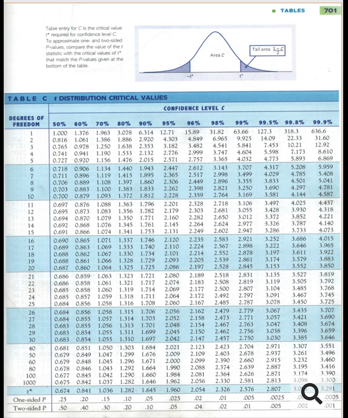
Table entry for C is the critical value
* required for confidence level C.
To approximate one- and two-sided
P-values, compare the value of the t
statistic with the critical values of t"
Tail area 15
Area C
that match the P-values given at the
bottom of the table.
TABLEC
t DISTRIBUTION CRITICAL VALUES
CONFIDENCE LEVEL C
DEGREES OF
FREEDOM
50%
60%
70%
80%
90%
95%
96%
98%
99%
99.5%
99.8%
99.9%
636.6
63.66
9.925
127.3
14.09
7.453
5.598
318.3
31.82
6.965
1.963
1.386
1.250
1.190
1.156
6.314
2.920
2.353
2.132
12.71
4.303
3.182
2.776
2.571
15.89
4.849
3.482
2.999
3.078
1.000
1.376
0.816
1.061
0.978
0.765
0.741
0.941
0.727 0.920
1
31.60
12.92
1.886
22.33
4.541
3.747
5.841
4.604
4.032
10.21
7.173
5.893
1.638
00.05
8.610
1.533
1.476
4
ILS 5
2.015
2.757
3.365
4.773
6.869
5.208
4.785
4.501
4.297
4.144
5.959
4.317
4.029
2.612
2.517
2.449
2.398
2.359
3.707
3.499
3.355
3.250
3.143
2.998
0.718 0.906
0.896
0.889
0.883
0.879
1.440
1.415
1.397
1.383
1.372
1.943
1.895
1.860
1.833
1.812
2.447
2.365
2.306
2.262
2.228
6.
1.134
5.408
5.041
4.781
4.587
7
0.711
1.119
2.896
2.821
2.764
3.833
8.
9.
0.706
0.703
0.700
1.108
1.100
3.690
3.581
10
1.093
3.169
2.718
2.681
2.650
2.624
3.106
3.055
3.012
2.977
2.947
3.497
3.428
3.372
4.025
3.930
3.852
3.787
3.733
4.437
4.318
4.221
4.140
1.363
1.356
1.796
1.782
2.201
2.179
2.160
2.145
2.328
0.697 0.876
0.695 0.873
0.694
0.692 0.868 1.076 1.345
0.691
11
1.088
12
1.083
2.303
2.282
2.264
2.249
13
0.870 1.079
1.350
1.771
14
1.761
3.326
15
0.866 1.074
1.341
1.753
2.131
2.602
3.286
4.073
4.015
3.965
3.922
3.883
3.850
3.252
3.222
3.686
3.646
3.611
3.579
2.921
2.898
1.746
1.740
1.734
2.235
2.224
2.214
2.583
2.567
2.552
2.539
2.528
2.120
0.865 1.071
1.069
1.067
1.066
1.064
1.337
0.690
0.689
16
2.110
0.863
0.862
17
1.333
2.878
2.861
2.845
18
0.688
1.330
2.101
3.197
2.093
2.086
3.174
3.153
2.205
1.328
1.325
1.729
1.725
19
0.688
0.861
20
0.687
0.860
2.197
3.552
3.527
3.505
3.485
3.467
3.450
3.819
3.792
3.768
3.745
3.725
3.135
2.189
2.183
2.518
2.508
2.500
2.492
2.485
2.831
1.323
1.321
1.319
1.721
1.717
1.714
1.711
1.708
2.080
2.074
2.069
2.064
0.686 0.859
0.858
0.686
1.063
1.061
2.819
3.119
22
GO.S23
3.104
1.060
1.059
1.058
2.177
2.172
2.167
2.807
2.797
2.787
0.685
0.858
1.318
3.091
0.685 0.857
0.684 0.856
24
25
1.316
2.060
3.078
3.435
3.421
3.408
3.396
3.385
2.779
3.067
3.707
1.706
1.703
1.701
1.699
1.697
2.162
2.158
2.154
2.150
2.479
2.473
2.467
2.462
2.457
1.058
1.057
1.315
1.314
1.313
2.056
0.684
0.684
0.683
0.856
0.855
26
3.690
3.057
3.047
2.771
2.052
2.048
2.045
2.042
27
2.763
2.756
3.674
3.659
3.646
28
0.855
1.056
1.311
3.038
0.854
0.854
1.055
29
30
0.683
0.683
1.055
1.310
2.147
2.750
3.030
3.551
2.971
2.937
3.307
3.261
1.050
1.047 1.299
0.679 0.848 1.045 1.296
0.846 1.043 1.292
1.042 1.290
1.037
1.684
1.676
1.671
1.664
1.660
1.646
2.123
2.109
2.099
2.088
2.081
2.056
2.423
2.403
2.390
2.374
2.364
2.330
2.704
2.678
2.660
2.639
2.626
1.303
2.021
0.681
0.679
0.851
40
50
60
80
100
1000
2.009
2.000
1.990
3.496
3.460
0.849
2.915
3.232
2.887
2.871
2.813
0.678
3.195
3.416
3.390
3.300
1.984
3.174
0.677 0.845
0.675
0.842
1.282
1.962
2.581
3.098
0.674
0.841
1.036
1.282 1.645
1.960
2.054
2.326
2.576
2.807
3.0
3.291
One-sided P
.25
.20
.15
.10
.05
.025
.02
.01
.005
.0025
.0005
Two-sided P
.50
.40
.30
.20
.10
.05
.04
.02
.01
.005
.002
.001
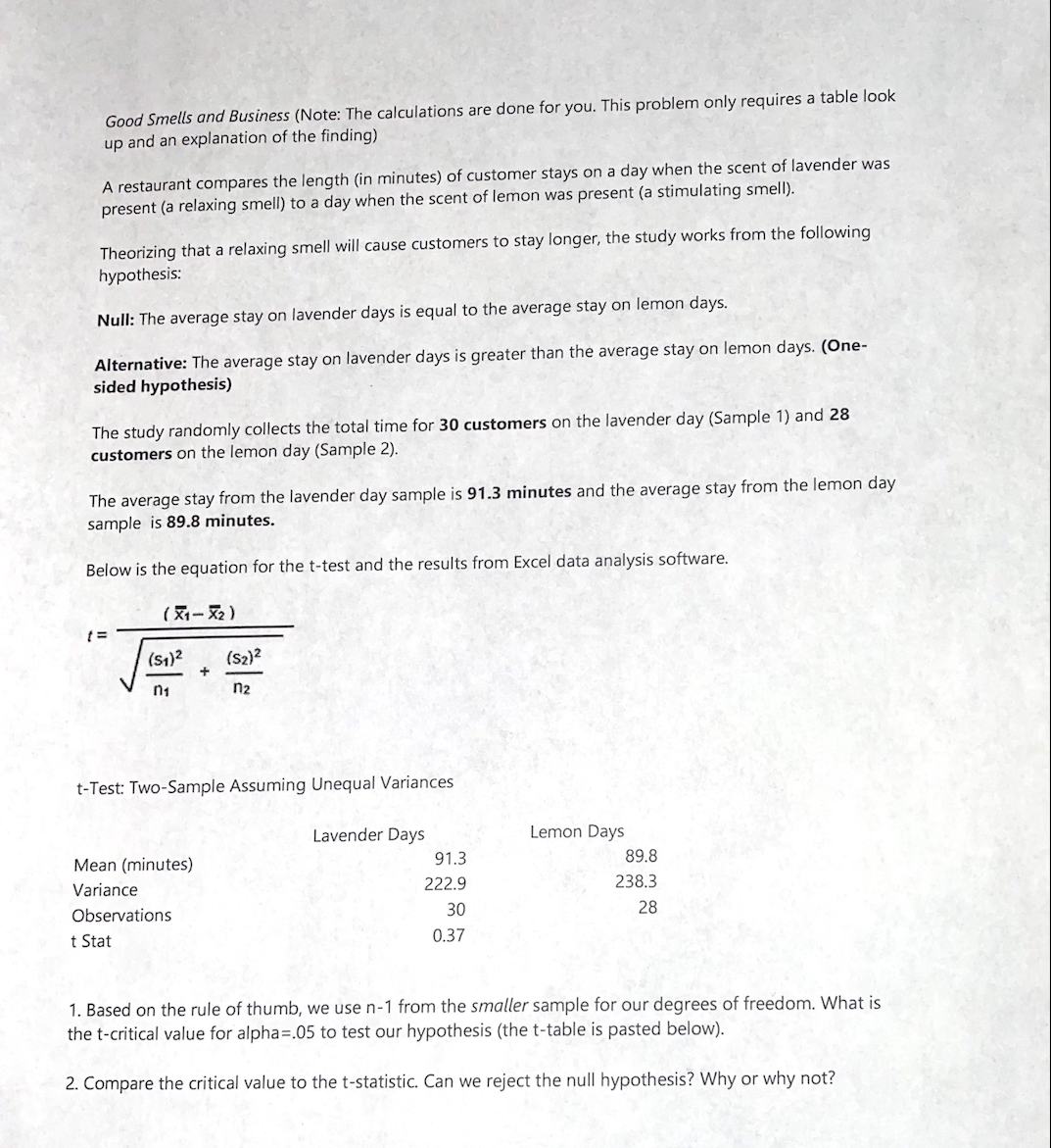
Transcribed Image Text:Good Smells and Business (Note: The calculations are done for you. This problem only requires a table look
up and an explanation of the finding)
A restaurant compares the length (in minutes) of customer stays on a day when the scent of lavender was
present (a relaxing smell) to a day when the scent of lemon was present (a stimulating smell).
Theorizing that a relaxing smell will cause customers to stay longer, the study works from the following
hypothesis:
Null: The average stay on lavender days is equal to the average stay on lemon days.
Alternative: The average stay on lavender days is greater than the average stay on lemon days. (One-
sided hypothesis)
The study randomly collects the total time for 30 customers on the lavender day (Sample 1) and 28
customers on the lemon day (Sample 2).
The average stay from the lavender day sample is 91.3 minutes and the average stay from the lemon day
sample is 89.8 minutes.
Below is the equation for the t-test and the results from Excel data analysis software.
(X- X2)
(s1)2
(s2)?
n1
n2
t-Test: Two-Sample Assuming Unequal Variances
Lavender Days
Lemon Days
Mean (minutes)
91.3
89.8
222.9
238.3
Variance
30
28
Observations
t Stat
0.37
1. Based on the rule of thumb, we use n-1 from the smaller sample for our degrees of freedom. What is
the t-critical value for alpha=.05 to test our hypothesis (the t-table is pasted below).
2. Compare the critical value to the t-statistic. Can we reject the null hypothesis? Why or why not?
Expert Solution
This question has been solved!
Explore an expertly crafted, step-by-step solution for a thorough understanding of key concepts.

This is a popular solution!

Trending now
This is a popular solution!

Step by step
Solved in 2 steps

Recommended textbooks for you
MATLAB: An Introduction with Applications
Statistics
ISBN:
9781119256830
Author:
Amos Gilat
Publisher:
John Wiley & Sons Inc

Probability and Statistics for Engineering and th…
Statistics
ISBN:
9781305251809
Author:
Jay L. Devore
Publisher:
Cengage Learning

Statistics for The Behavioral Sciences (MindTap C…
Statistics
ISBN:
9781305504912
Author:
Frederick J Gravetter, Larry B. Wallnau
Publisher:
Cengage Learning
MATLAB: An Introduction with Applications
Statistics
ISBN:
9781119256830
Author:
Amos Gilat
Publisher:
John Wiley & Sons Inc
Probability and Statistics for Engineering and th…
Statistics
ISBN:
9781305251809
Author:
Jay L. Devore
Publisher:
Cengage Learning
Statistics for The Behavioral Sciences (MindTap C…
Statistics
ISBN:
9781305504912
Author:
Frederick J Gravetter, Larry B. Wallnau
Publisher:
Cengage Learning

Elementary Statistics: Picturing the World (7th E…
Statistics
ISBN:
9780134683416
Author:
Ron Larson, Betsy Farber
Publisher:
PEARSON

The Basic Practice of Statistics
Statistics
ISBN:
9781319042578
Author:
David S. Moore, William I. Notz, Michael A. Fligner
Publisher:
W. H. Freeman

Introduction to the Practice of Statistics
Statistics
ISBN:
9781319013387
Author:
David S. Moore, George P. McCabe, Bruce A. Craig
Publisher:
W. H. Freeman