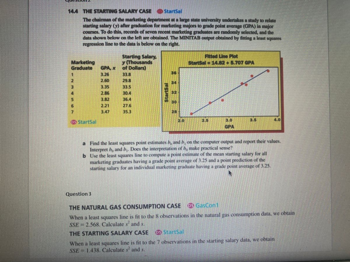
144 THE STARTING SALARY CASEStartsalThe chairman of the marketing department at a large state university undertakes a study to relatestarting salary (y) after graduation for marketing majors to grade point average (GPA) in majorcourses. To do this, records of seven recent marketing graduates are randomly selected, and thedata shown below on the left are obtained. The MINITAB output obtained by fitting a least squaresregression line to the data is below on the right.Starting Salary,Fitted Line PlotMarketingy (ThousandsStartSal= 14.82 +5.707 GPAGraduate GPA, x of Dollars)13.2633.82.6029.833.52,8630.43.8236.42.2127.63.4735.3de Startsal2.02.5aFind the least squares point estimates b, and b, on the computer output and report their values.Interpret b, and b,. Does the interpretation of b, make practical sense?bUse the least squares line to compute a point estimate of the mean starting salary for allmarketing graduates having a grade point average of 3.25 and a point prediction of thestarting salary for an individual marketing graduate having a grade point average of 3.25.Question 3THE NATURAL GAS CONSUMPTION CASE OS GasCon1When a least squares line is fit to the 8 observations in the natural gas consumption data, we obtainSSE 2.568. Calculates and s.THE STARTING SALARY CASE 5 Starts.When a least squares line is fit to the 7 observations in the starting salary data, we obtainSSE 1.438. Calculates and s.235PJespers28

Given, The chairman of the marketing department at a large state university undertakes a stdy to…

Answered: 14.4 THE STARTING SALARY CASE StartSal…

MATLAB: An Introduction with Applications

6th Edition

ISBN:9781119256830

Author:Amos Gilat

Publisher:Amos Gilat

Chapter1: Starting With Matlab

Section: Chapter Questions

Problem 1P

See similar textbooks

Similar questions

The article “Characterization of Highway Runoff in Austin, Texas, Area” (J. of Envir. Engr., 1998: 131–137) gave a scatterplot, along with the least squares line, of x = rainfall volume (m3) and y = runoff volume (m3) for a particular location. The accompanying values were read from the plot. x <‐ c(5, 12, 14, 17, 23, 30, 40, 47, 55, 67, 72, 81, 96, 112, 127) y <‐ c(4, 10, 13, 15, 15, 25, 27, 46, 38, 46, 53, 70, 82, 99, 100) Test at level 0.05 whether there is a useful linear relationship between rainfall and runoff,and then calculate a 95% confidence interval for the true average change in runoff volumeassociated with one unit (one m3) increase in rainfall volume.
In Austria ,The amount of money spent on the restoration of a sanctuary and the distinct kangaroo populations present appeared to have negative correlations For investigation of this onserved assocaition ,what can a resecher do to begin his research 1Conduct an experiment 2Calculate the squares of coreealtion coefficient 3Calculate the least squares regression line 4 calculate the corelation coefficient Explain answer in 1 or 2 lines
One important aspect of medical diagnosis is its reproducibility. Suppose that two different doctors examine 100 patients for dyspnea in a respiratory-disease clinic and that doctor A diagnosed 15 patients as having dyspnea, doctor B diagnosed 10 patients as having dyspnea, and both doctor A and doctor B diagnosed 7 patients as having dyspnea. Compute the Kappa statistic and its standard error regarding reproducibility of the diagnosis of dyspnea in this clinic.
Calculate Pearson’s coefficient of skewness. Hence, describe the shape of thedistribution of the waiting time for counter A and B.
At 5% level of significance, test if the Penicillium roqueforti colonies grown on malt extract agar are bigger than when grown on Czapek yeast autolysate agar using the given R-software output:Fill-up the following as the answer: Ho, Ha,Test procedure, Decision Rule, Computed test statistic and p-value, Decision, Conclusion
A manufacturer of sunflower oil uses machines to distribute liquid ingredients into bottles that move along a filling line. The machine that distributes is working properly when 8 ounces are distributed Suppose that the average amount distributed in a particular sample of 35 bottles is 7 91 0 ounces. Assume that the variance of the process is known to be 0.03 ounces squared. Is there evidence that the machine should be stopped (when not 8 ounces are distributed), and production wait for repairs? The lost production from a shutdown is potentially so great that management feels that the level of confidence in the analysis should be 99%
Test the hypothesis that the average weekly allowance of female and male ACC 215 students the same, at 5%l evel of significance. (Step by step solution, manually, without using excel) Weekly Allowance of Students (Php) Male: 1500 2000 2500 2500 2000 1750 2000 1800 Female:1500 2000 1750 1500 2000 2500 3000 3500 Ho: Ha: α = Decision Rule: Computation: Decision: Conclusion:
A high school principal wanted to know if there was a difference in absences for 9th grade, 10th grade, 11th grade, and 12th grade among students with less than a 2.0 GPA. She took a random sample of n=5 students from each grade level and compared absences among the four grades using ANOVA. 9th grade 10th grade 11th grade 12th grade 6 10 17 15 9 12 8 16 6 11 11 12 7 11 14 12 7 14 15 12 Calculate the sum of squares within…
A scatterplot of student height, in inches, versus corresponding arm span length, in inches, is shown below. One of the points in the graph is labeled A. If the point labeled A is removed, which of the following statements would be true? The slope of the least squares regression line is unchanged and the correlation coefficient increases. The slope of the least squares regression line is unchanged and the correlation coefficient decreases. The slope of the least squares regression line increases and the correlation coefficient increases. The slope of the least squares regression line increases and the correlation coefficient decreases. The slope of the least squares regression line decreases and the correlation coefficient increases.
The shape of the mean-variance frontier that results from the combination of a riskless and arisky asset is…..:a. Is U-shaped, tilted 90 degrees clockwise.b. Is a straight line passing from the mean-variance points of the two assets.c. Is a hyperbola.d. Consists of two straight lines, each connecting one of the two assets to a risk-freeportfolio
J 2 make a 2 way ANOVA table for data on MATLAB with code
A Department of Psychology professor conducts an experiment that investigates the effect of gender (male vs. female) and time pressure (30 minutes, 50 minutes, 70 minutes and 90 minutes) on exam performance. After running some numbers, he computes the following sums of squares for a between groups factorial ANOVA (n = 30 and N = 120). Please complete the ANOVA summary table above and indicate whether the p values for the main effect of gender (pgender), the main effect of time pressure (pcondition) and the gender by time pressure interaction (pgenderXcondition) are "significant" or "not significant" at α = .05. Please make sure to round your answers to two decimal points.

SEE MORE QUESTIONS

Recommended textbooks for you

MATLAB: An Introduction with Applications

Statistics

ISBN:

9781119256830

Author:

Amos Gilat

Publisher:

John Wiley & Sons Inc

Probability and Statistics for Engineering and th…

Statistics

ISBN:

9781305251809

Author:

Jay L. Devore

Publisher:

Cengage Learning

Statistics for The Behavioral Sciences (MindTap C…

Statistics

ISBN:

9781305504912

Author:

Frederick J Gravetter, Larry B. Wallnau

Publisher:

Cengage Learning

MATLAB: An Introduction with Applications

Statistics

ISBN:

9781119256830

Author:

Amos Gilat

Publisher:

John Wiley & Sons Inc

Probability and Statistics for Engineering and th…

Statistics

ISBN:

9781305251809

Author:

Jay L. Devore

Publisher:

Cengage Learning

Statistics for The Behavioral Sciences (MindTap C…

Statistics

ISBN:

9781305504912

Author:

Frederick J Gravetter, Larry B. Wallnau

Publisher:

Cengage Learning

Elementary Statistics: Picturing the World (7th E…

Statistics

ISBN:

9780134683416

Author:

Ron Larson, Betsy Farber

Publisher:

PEARSON

The Basic Practice of Statistics

Statistics

ISBN:

9781319042578

Author:

David S. Moore, William I. Notz, Michael A. Fligner

Publisher:

W. H. Freeman

Introduction to the Practice of Statistics

Statistics

ISBN:

9781319013387

Author:

David S. Moore, George P. McCabe, Bruce A. Craig

Publisher:

W. H. Freeman

SEE MORE TEXTBOOKS