4. The STATA output below uses the Educational Attainment and Wage Equations (EAWE) data similar to what we have investigated in class: reg EARNINGS S FEMALE ASVABC ETHHISP ETHWHITE MARRIED EXP TENURE 500 Source | df Number of obs SS MS omitted F (8, 491) Model | 11567.0578 8. omitted Prob > F omitted omitted Residual 55379.8233 491 R-squared Adj R-squared 0.1728 0.1593 Total | 10.62 66946.8811 499 134.162086 Root MSE P> |t| EARNINGS | Std. Err. [95% Conf. Interval] Coef. 5.13 1.282268 .2499762 0.000 .7911128 1.773423 0.012 -.5480824 3.428481 FEMALE | ASVABC | -2.457466 .9717918 -2.53 -4.36685 2.206915 .6217233 3.55 0.000 .9853484 1.985396 0.685 3.094036 ETHHISP -.8068838 -0.41 -4.707804 ETHWHITE | MARRIED | 1.670643 -0.98 0.329 -1.63153 -4.91402 1.650961 1.720857 .9850864 1.75 0.081 -.2146475 3.656362 . 4396207 EXP | 3.99 .8659335 .2169744 0.000 1.292246 .3597575 .1895722 1.90 0.058 -.0127153 .7322303 TENURE -6.210424 2.704951 4.537532 -1.37 0.172 -15.1258 cons Assume the true model of the relationship is EARNINGS = ß1 + B2S + B3FEMALE + B4ASV ABC + В-ЕТНHISP + BsЕТHWHITE + B-MARRIED + B3EXP + B9TENURE + u where EARNINGS is hourly earnings in dollars, S is years of schooling, FEMALE is a dummy variable for women, ASVABC is a measure of cognitive ability, ETHHISP is a dummy for Hispanic people, ETHWHITE is a dummy for White people, MARRIED is a dummy variable for the married, EXP is of job experience after the graduation, and TENURE is years after one's job was tenured. (to.05,491 years = 1.6479629 to.025,491 1.9648027, and Fo.05(8, 491) = 1.9572532) Interpret the estimated coefficients. (Answer briefly) Based on the regression output above, are there any differences in hourly earnings by race? Based on the regression output above, are there any differences in hourly earnings by gender? Test the overall significance of the regression model at the 5% level of significance. Define the relevant hypotheses and compute the F-statistic for the test. What would be the conclusion of the test? Explain the result. How do you check the heteroskedasticity? Explain the relevant test procedure with the model above. (a) (b) (c) (d) (e) (f) Assume that you detected the heteroskedasticity from the given regression model. How can you possibly resolve the problem? Explain.
4. The STATA output below uses the Educational Attainment and Wage Equations (EAWE) data similar to what we have investigated in class: reg EARNINGS S FEMALE ASVABC ETHHISP ETHWHITE MARRIED EXP TENURE 500 Source | df Number of obs SS MS omitted F (8, 491) Model | 11567.0578 8. omitted Prob > F omitted omitted Residual 55379.8233 491 R-squared Adj R-squared 0.1728 0.1593 Total | 10.62 66946.8811 499 134.162086 Root MSE P> |t| EARNINGS | Std. Err. [95% Conf. Interval] Coef. 5.13 1.282268 .2499762 0.000 .7911128 1.773423 0.012 -.5480824 3.428481 FEMALE | ASVABC | -2.457466 .9717918 -2.53 -4.36685 2.206915 .6217233 3.55 0.000 .9853484 1.985396 0.685 3.094036 ETHHISP -.8068838 -0.41 -4.707804 ETHWHITE | MARRIED | 1.670643 -0.98 0.329 -1.63153 -4.91402 1.650961 1.720857 .9850864 1.75 0.081 -.2146475 3.656362 . 4396207 EXP | 3.99 .8659335 .2169744 0.000 1.292246 .3597575 .1895722 1.90 0.058 -.0127153 .7322303 TENURE -6.210424 2.704951 4.537532 -1.37 0.172 -15.1258 cons Assume the true model of the relationship is EARNINGS = ß1 + B2S + B3FEMALE + B4ASV ABC + В-ЕТНHISP + BsЕТHWHITE + B-MARRIED + B3EXP + B9TENURE + u where EARNINGS is hourly earnings in dollars, S is years of schooling, FEMALE is a dummy variable for women, ASVABC is a measure of cognitive ability, ETHHISP is a dummy for Hispanic people, ETHWHITE is a dummy for White people, MARRIED is a dummy variable for the married, EXP is of job experience after the graduation, and TENURE is years after one's job was tenured. (to.05,491 years = 1.6479629 to.025,491 1.9648027, and Fo.05(8, 491) = 1.9572532) Interpret the estimated coefficients. (Answer briefly) Based on the regression output above, are there any differences in hourly earnings by race? Based on the regression output above, are there any differences in hourly earnings by gender? Test the overall significance of the regression model at the 5% level of significance. Define the relevant hypotheses and compute the F-statistic for the test. What would be the conclusion of the test? Explain the result. How do you check the heteroskedasticity? Explain the relevant test procedure with the model above. (a) (b) (c) (d) (e) (f) Assume that you detected the heteroskedasticity from the given regression model. How can you possibly resolve the problem? Explain.

Glencoe Algebra 1, Student Edition, 9780079039897, 0079039898, 2018
18th Edition
ISBN:9780079039897
Author:Carter
Publisher:Carter
Chapter10: Statistics
Section10.3: Measures Of Spread
Problem 1GP

Related questions
Question
![4. The STATA output below uses the Educational Attainment and Wage Equations (EAWE) data similar to
what we have investigated in class:
reg EARNINGS S FEMALE ASVABC ETHHISP ETHWHITE MARRIED EXP TENURE
500
Source |
df
Number of obs
SS
MS
omitted
F (8, 491)
Model |
11567.0578
8.
omitted
Prob > F
omitted
omitted
Residual
55379.8233
491
R-squared
Adj R-squared
0.1728
0.1593
Total |
10.62
66946.8811
499
134.162086
Root MSE
P> |t|
EARNINGS |
Std. Err.
[95% Conf. Interval]
Coef.
5.13
1.282268
.2499762
0.000
.7911128
1.773423
0.012
-.5480824
3.428481
FEMALE |
ASVABC |
-2.457466
.9717918
-2.53
-4.36685
2.206915
.6217233
3.55
0.000
.9853484
1.985396
0.685
3.094036
ETHHISP
-.8068838
-0.41
-4.707804
ETHWHITE |
MARRIED |
1.670643
-0.98
0.329
-1.63153
-4.91402
1.650961
1.720857
.9850864
1.75
0.081
-.2146475
3.656362
. 4396207
EXP |
3.99
.8659335
.2169744
0.000
1.292246
.3597575
.1895722
1.90
0.058
-.0127153
.7322303
TENURE
-6.210424
2.704951
4.537532
-1.37
0.172
-15.1258
cons](/v2/_next/image?url=https%3A%2F%2Fcontent.bartleby.com%2Fqna-images%2Fquestion%2F68d47df5-7aa7-45b3-90d4-b84567680c3f%2Fbbe48512-fc2a-4303-a464-71068fb8b568%2Fzootwlq.png&w=3840&q=75)
Transcribed Image Text:4. The STATA output below uses the Educational Attainment and Wage Equations (EAWE) data similar to
what we have investigated in class:
reg EARNINGS S FEMALE ASVABC ETHHISP ETHWHITE MARRIED EXP TENURE
500
Source |
df
Number of obs
SS
MS
omitted
F (8, 491)
Model |
11567.0578
8.
omitted
Prob > F
omitted
omitted
Residual
55379.8233
491
R-squared
Adj R-squared
0.1728
0.1593
Total |
10.62
66946.8811
499
134.162086
Root MSE
P> |t|
EARNINGS |
Std. Err.
[95% Conf. Interval]
Coef.
5.13
1.282268
.2499762
0.000
.7911128
1.773423
0.012
-.5480824
3.428481
FEMALE |
ASVABC |
-2.457466
.9717918
-2.53
-4.36685
2.206915
.6217233
3.55
0.000
.9853484
1.985396
0.685
3.094036
ETHHISP
-.8068838
-0.41
-4.707804
ETHWHITE |
MARRIED |
1.670643
-0.98
0.329
-1.63153
-4.91402
1.650961
1.720857
.9850864
1.75
0.081
-.2146475
3.656362
. 4396207
EXP |
3.99
.8659335
.2169744
0.000
1.292246
.3597575
.1895722
1.90
0.058
-.0127153
.7322303
TENURE
-6.210424
2.704951
4.537532
-1.37
0.172
-15.1258
cons
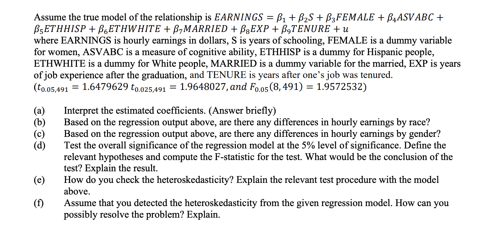
Transcribed Image Text:Assume the true model of the relationship is EARNINGS = ß1 + B2S + B3FEMALE + B4ASV ABC +
В-ЕТНHISP + BsЕТHWHITE + B-MARRIED + B3EXP + B9TENURE + u
where EARNINGS is hourly earnings in dollars, S is years of schooling, FEMALE is a dummy variable
for women, ASVABC is a measure of cognitive ability, ETHHISP is a dummy for Hispanic people,
ETHWHITE is a dummy for White people, MARRIED is a dummy variable for the married, EXP is
of job experience after the graduation, and TENURE is years after one's job was tenured.
(to.05,491
years
= 1.6479629 to.025,491
1.9648027, and Fo.05(8, 491) = 1.9572532)
Interpret the estimated coefficients. (Answer briefly)
Based on the regression output above, are there any differences in hourly earnings by race?
Based on the regression output above, are there any differences in hourly earnings by gender?
Test the overall significance of the regression model at the 5% level of significance. Define the
relevant hypotheses and compute the F-statistic for the test. What would be the conclusion of the
test? Explain the result.
How do you check the heteroskedasticity? Explain the relevant test procedure with the model
above.
(a)
(b)
(c)
(d)
(e)
(f)
Assume that you detected the heteroskedasticity from the given regression model. How can you
possibly resolve the problem? Explain.
Expert Solution
This question has been solved!
Explore an expertly crafted, step-by-step solution for a thorough understanding of key concepts.

This is a popular solution!

Trending now
This is a popular solution!

Step by step
Solved in 4 steps with 1 images

Recommended textbooks for you
Glencoe Algebra 1, Student Edition, 9780079039897…
Algebra
ISBN:
9780079039897
Author:
Carter
Publisher:
McGraw Hill
Glencoe Algebra 1, Student Edition, 9780079039897…
Algebra
ISBN:
9780079039897
Author:
Carter
Publisher:
McGraw Hill